
 Submit a Paper
 Propose a Special lssue
 Open Access
REVIEW
Gait Planning, and Motion Control Methods for Quadruped Robots: Achieving High Environmental Adaptability: A Review
School of Electrical and Control Engineering, Shaanxi University of Science and Technology, Xi’an, 710016, China
* Corresponding Author: Sheng Dong. Email:
(This article belongs to the Special Issue: Environment Modeling for Applications of Mobile Robots)
Computer Modeling in Engineering & Sciences 2025, 143(1), 1-50. https://doi.org/10.32604/cmes.2025.062113
Received 10 December 2024; Accepted 17 February 2025; Issue published 11 April 2025
 View Full Text
 Download PDF
Abstract
Legged robots have always been a focal point of research for scholars domestically and internationally. Compared to other types of robots, quadruped robots exhibit superior balance and stability, enabling them to adapt effectively to diverse environments and traverse rugged terrains. This makes them well-suited for applications such as search and rescue, exploration, and transportation, with strong environmental adaptability, high flexibility, and broad application prospects. This paper discusses the current state of research on quadruped robots in terms of development status, gait trajectory planning methods, motion control strategies, reinforcement learning applications, and control algorithm integration. It highlights advancements in modeling, optimization, control, and data-driven approaches. The study identifies the adoption of efficient gait planning algorithms, the integration of reinforcement learning-based control technologies, and data-driven methods as key directions for the development of quadruped robots. The aim is to provide theoretical references for researchers in the field of quadruped robotics.Keywords
Science and technology are advancing rapidly, and the application fields of robots are gradually expanding, with increasing demands for their functionality [1–3]. Various types of robots are gradually entering the public’s view [4]. Due to the large stability domain and simple structure of quadruped robots [5–7], they have more research value and significance compared to other legged robots. Generally speaking, the drive methods for quadruped robots are divided into two categories [8]: hydraulic drive and motor drive. Motor drives make it easier to achieve precise speed and position control, with a simple mechanical structure that is convenient for maintenance and operation, but it carries a relatively small load [9]. Hydraulic drive can provide greater force, making it suitable for heavy-duty and high-intensity tasks, but the hydraulic system is complex, and maintenance and repair are relatively difficult [10].
The development of quadruped robots can be roughly divided into five stages: the mechanical fundamentals stage, the theoretical foundation and experimental research stage, the intelligent exploration stage, the bionics and efficiency stage, and the application and commercialization stage.
The First Stage—Mechanical Fundamentals Stage: Research on quadruped robots can be traced back to the late 19th century, focusing primarily on mechanical drive systems and the exploration of simple gaits. In 1870, Chebyshev designed the world’s first quadruped robot. This robot utilized a crank-rocker mechanism, with its four legs performing diagonal synchronized movements. Although it had only one degree of freedom and could not handle complex terrains, its mechanical design provided an initial framework for the realization of quadruped robots [11]. In the 1960s, robot technology experienced a new wave of development opportunities with the rise of computer science. In 1966, McGhee and Frank at the University of California developed the world’s first computer-controlled quadruped robot, the Phony Pony. This robot featured eight degrees of freedom and, for the first time, used electric motors as the power source, with a computer controlling leg movements. This design laid an important foundation for subsequent research into automated gaits for quadruped robots [12]. To promote the transition from mechanical technology to intelligence, research during this stage focused on structural optimization and drive methods. For example, in 1968, General Electric and the U.S. Army collaborated to develop a hydraulically driven walking vehicle, which not only achieved breakthroughs in load capacity but also enabled flexible mechanical legs to overcome obstacles. Although research during this period was primarily centered on hardware development, it established the foundational framework for quadruped robot research [13].
The Second Stage—Theoretical Foundation and Experimental Research: With advances in computing technology, research on quadruped robots gradually moved towards a combination of theory and practice. In the 1970s, Professor Hirose from the Tokyo Institute of Technology designed the KUMO-I robot, which was the first to integrate bionic design with gravity decoupling methods. By equipping the robot with tactile sensors and a posture control system, it achieved basic terrain adaptation capabilities [14]. At the same time, McGhee further proposed a scientific definition of gait, clarifying key parameters such as stride length, phase, and duty cycle. These parameters not only provided a standardized framework for robot gait analysis but also offered theoretical support for optimizing the gait of multi-legged robots [15,16]. During this stage, various gait planning algorithms began to emerge, including static gaits, dynamic gaits, and optimized diagonal gaits. Taking static gaits as an example, quantifiable modeling of each leg’s support time and relative movement was implemented, enhancing the robot’s stability on flat terrain [17,18]. The research achievements of this period laid a solid theoretical foundation for subsequent control methods based on dynamic models.
The Third Stage—Exploration of Intelligence: In the 1980s, with the gradual maturation of sensor technology and the application of embedded systems, quadruped robots entered the stage of intelligent exploration. The Tokyo Institute of Technology introduced the TITAN series robots, particularly the TITAN VIII, which featured a high-efficiency chain drive in its mechanical structure. It also integrated tactile sensors, accelerometers, and a visual feedback system. Its intelligent control capabilities enabled it to accomplish complex tasks such as demining and load carrying [19]. Research during this stage also focused on environmental perception and real-time path planning. By integrating the robot with external sensor networks, the TITAN series demonstrated exceptional performance in obstacle crossing and navigating unstructured terrains [20].
The Fourth Stage—Bionics and Efficiency: In the early 21st century, research on quadruped robots advanced further towards bionic design and high efficiency. In 2005, Boston Dynamics released BigDog, which became a hallmark achievement of this stage. As a hydraulically driven robot, BigDog demonstrated impressive load-carrying and balancing capabilities on complex terrains. By integrating bionic principles with dynamic models, BigDog achieved dynamic pressure adjustments on its footpads, significantly improving stability and energy efficiency [21]. In 2008, Boston Dynamics introduced the second-generation BigDog [22], resembling the size of a large dog or small mule. Weighing approximately 109 kg, with a height of 1 m, a length of 1.1 m, and a width of 0.3 m, it could carry loads of up to 154 kg on flat terrain. The second-generation BigDog was equipped with four active joints per leg, totaling 16 active joints, all driven by a hydraulic servo system. Its power source was an onboard internal combustion engine. The robot could execute a crawling gait at a speed of about 0.2 m/s, a diagonal trot at 2 m/s, and even a jumping gait in laboratory settings, reaching speeds of over 3.1 m/s. What made BigDog particularly remarkable was its superior locomotion capabilities and terrain adaptability. It could jump 1.1 m high, climb steep slopes of up to 35°, and traverse challenging terrains such as mountains, jungles, icy surfaces, and snow. Subsequently, Boston Dynamics introduced the smaller and more agile LittleDog. This robot weighed only 2.85 kg, measured 34 cm in length and 18.5 cm in width, and was powered by a lithium-polymer battery. Supporting the remote control, LittleDog could navigate rocky terrains and operate for up to 30 min.
The Fifth Stage—Application and Commercialization: After 2010, quadruped robots entered the stage of application and commercialization. Boston Dynamics’ Spot series, through modular design and intelligent control algorithms, quickly became a leading solution for complex terrain inspection and logistics handling [23]. Among them, SpotMini stood out for its lightness and flexibility, excelling in commercial environments and further driving the application of quadruped robots in the service industry [24]. Subsequently, Boston Dynamics released SpotMini, a fully electric-driven quadruped robot equipped with a mechanical arm and gripping device, along with a sophisticated autonomous navigation system capable of mapping and quickly performing simple repetitive tasks. In 2017, after two years of optimization, SpotMini2 was introduced as an all-electric driven robot. Thanks to its agile “limbs” and lightweight mobility, it quickly attracted attention. SpotMini2 can easily navigate stairs, and complex terrains, and autonomously patrol using lidar and visual cameras. It is suitable for various commercial applications, such as power inspection and complex environment search [25]. The StarlETH robot from ETH Zurich in Switzerland used series elastic actuation (SEA) technology for precise torque control and compliant movement. Based on this, the ANYmal series robots further integrated SEA with global motion planning, finding widespread use in industrial inspections, search and rescue, and the energy sector [26,27]. In addition, MIT’s Cheetah series robots focused on breakthroughs in extreme performance [28]. In terms of high-speed running and jumping abilities, the Cheetah robots showcased unmatched technical advantages and achieved efficient ground reaction force utilization through improved foot structures [29]. Meanwhile, Chinese companies also began to make their mark in this field. Since its establishment in 2016, Unitree Robotics has rapidly advanced quadruped robot technology, thanks to the technical accumulation of its founder, Wang Xingxing. In 2017, Unitree Robotics launched Laikago, the first quadruped robot for educational and research purposes, widely used in motion control research [30]. Later, Unitree released higher-performance robots, including the A1 in 2020, which achieved a speed of 3.3 m/s and demonstrated excellent dynamic balance capabilities [31]. By 2021, Unitree released the B1, the world’s first industrial-grade quadruped robot, capable of carrying a maximum load of 80 kg and adaptable to complex environments such as stairs and rubble [32]. Additionally, Go1 became a smart robot for daily applications such as companionship and guide dogs [33]. Yunshenchu Technology’s Jueying series also made breakthroughs in the field of quadruped robots. From 2018 to 2021, Yunshenchu released several robots, including the Jueying Mini, which weighs 23 kg and has a load capacity of 10 kg, widely used in education, research, and competition scenarios. The larger versions of the Jueying robot have a stronger load-bearing capacity and can adapt to various complex terrains, such as stairs, grass, and snow, with excellent self-adaptive capabilities [34,35]. The latest Jueying X20 model weighs 50 kg and is capable of performing hazardous tasks like power inspection and firefighting reconnaissance [36]. The development of quadruped robots is shown in Fig. 1, spanning from mechanical drive to intelligent control, and from theoretical research to practical application. In the future, as artificial intelligence and robotics further converge, quadruped robots will make significant breakthroughs in efficiency, energy conservation, and multifunctionality, bringing more possibilities for various application scenarios.
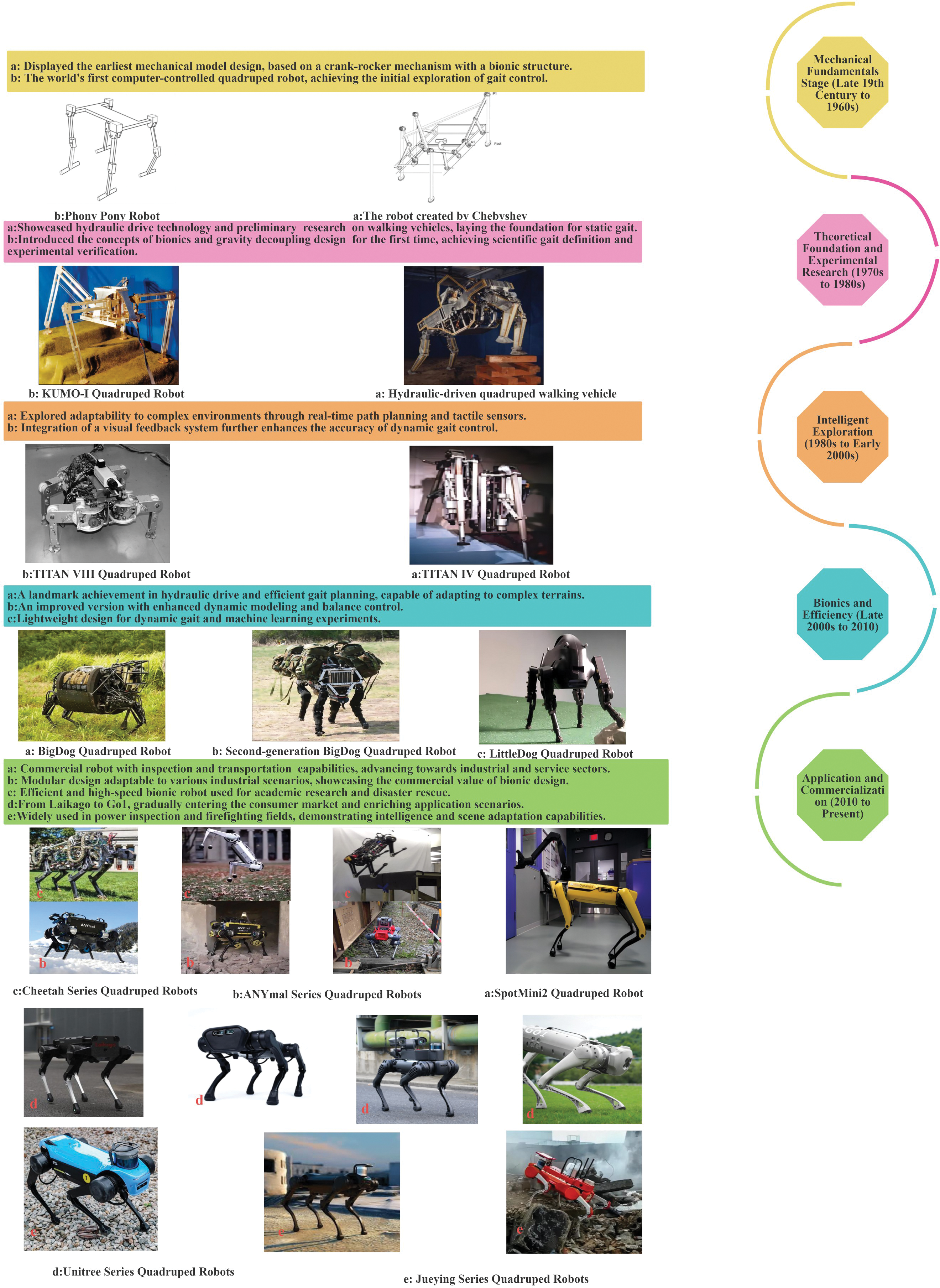
Figure 1: The development history of quadruped robots
As mentioned above, quadruped robots can adapt to various complex environments, making their application prospects very broad [37]. They cover multiple fields, primarily including the following areas:
Military and Security: Used for tasks such as reconnaissance, surveillance, and mine clearance, quadruped robots are capable of performing high-risk operations in complex environments.
Border Patrol: In high-altitude areas, patrol efficiency is often limited by physiological factors like altitude sickness. Quadruped robots, with their excellent terrain adaptability [38], can be equipped with environmental sensing devices, generate high-precision maps in all weather conditions, and effectively identify and detect suspicious individuals. Therefore, they have a clear advantage in border patrol and can effectively replace humans in executing these tasks.
Emotional Companionship: Quadruped robots show great potential in family life applications. They can be equipped with navigation systems for autonomous movement, engage in emotional communication with family members through speech and gestures, participate in interactive games, and even perform activities such as dance.
Search and Rescue: In post-disaster environments such as earthquakes and floods, quadruped robots can traverse rubble to conduct life detection [39] and transport supplies.
Therefore, the development of quadruped robots is not only a critical foundation for emerging industries and a core direction for future technological advancements but also an important part of human societal progress, widely serving the national economy and defense construction. However, to fully leverage the adaptability and functionality of quadruped robots in complex environments, gait planning and motion control technologies are crucial. These technologies not only determine the robot’s movement efficiency and stability but also directly impact its ability to complete tasks in dynamic, unstructured environments. As a result, in-depth research and optimization of gait planning and motion control methods, as well as the exploration of diverse algorithm designs and control strategies, will provide robust technical support for the practical application of quadruped robots in various fields.
2 Model-Based Planning/Optimization Methods for Quadruped Robots
Waldron defined gait precisely in 1989 as how a robot moves its legs in a specific sequence during motion [40]. In the natural world, legged animals choose appropriate gaits based on different terrain conditions and survival environments [41], thereby improving their adaptability to the environment. For legged robots, gait planning is the core of motion control and defines how the quadruped robot moves. Proper gait planning can reduce the impact of the foot on the ground [42], thereby minimizing damage to the robot. Different gait patterns have a significant impact on the robot’s motion stability and speed, serving as an important basis for determining whether the quadruped robot can operate stably [43] and complete tasks effectively.
2.1 Definition of Gait Parameters
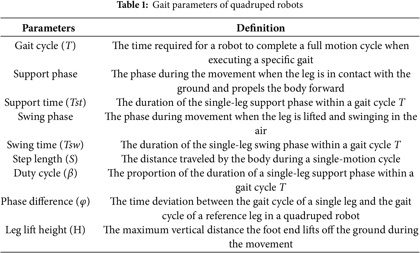
The gait of a quadruped robot is a complex leg movement that involves multiple gait parameters such as leg support, swing, and phase differences [44]. These parameters are key indicators that describe its walking pattern and are crucial for the robot’s motion control and behavioral performance. By adjusting the gait parameters, the gait pattern of the quadruped robot can be optimized, improving its movement efficiency, stability, and adaptability. Table 1 provides an introduction to each gait parameter.
The gait cycle, step length, and duty cycle of a quadruped robot are interrelated and mutually influential. When planning the gait of a quadruped robot, these three relationships must be considered. The specific relationships are shown in Eq. (1).
where v: Running speed.
The gait characteristics of a quadruped robot [45] are determined by the duty cycle β and phase difference
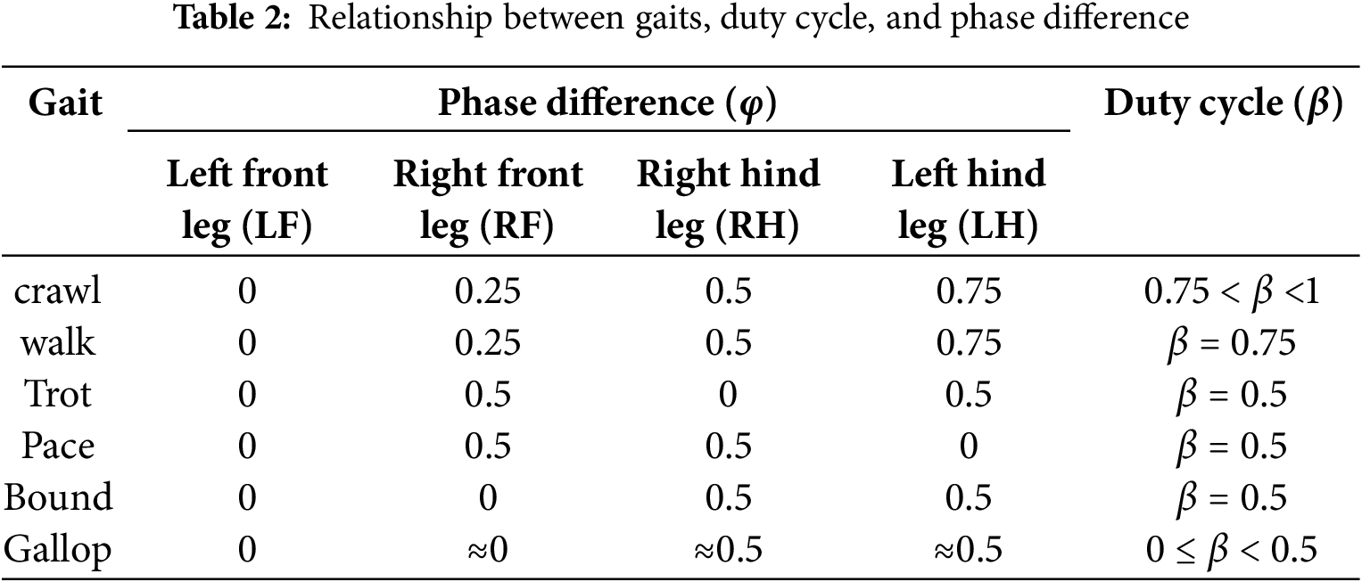
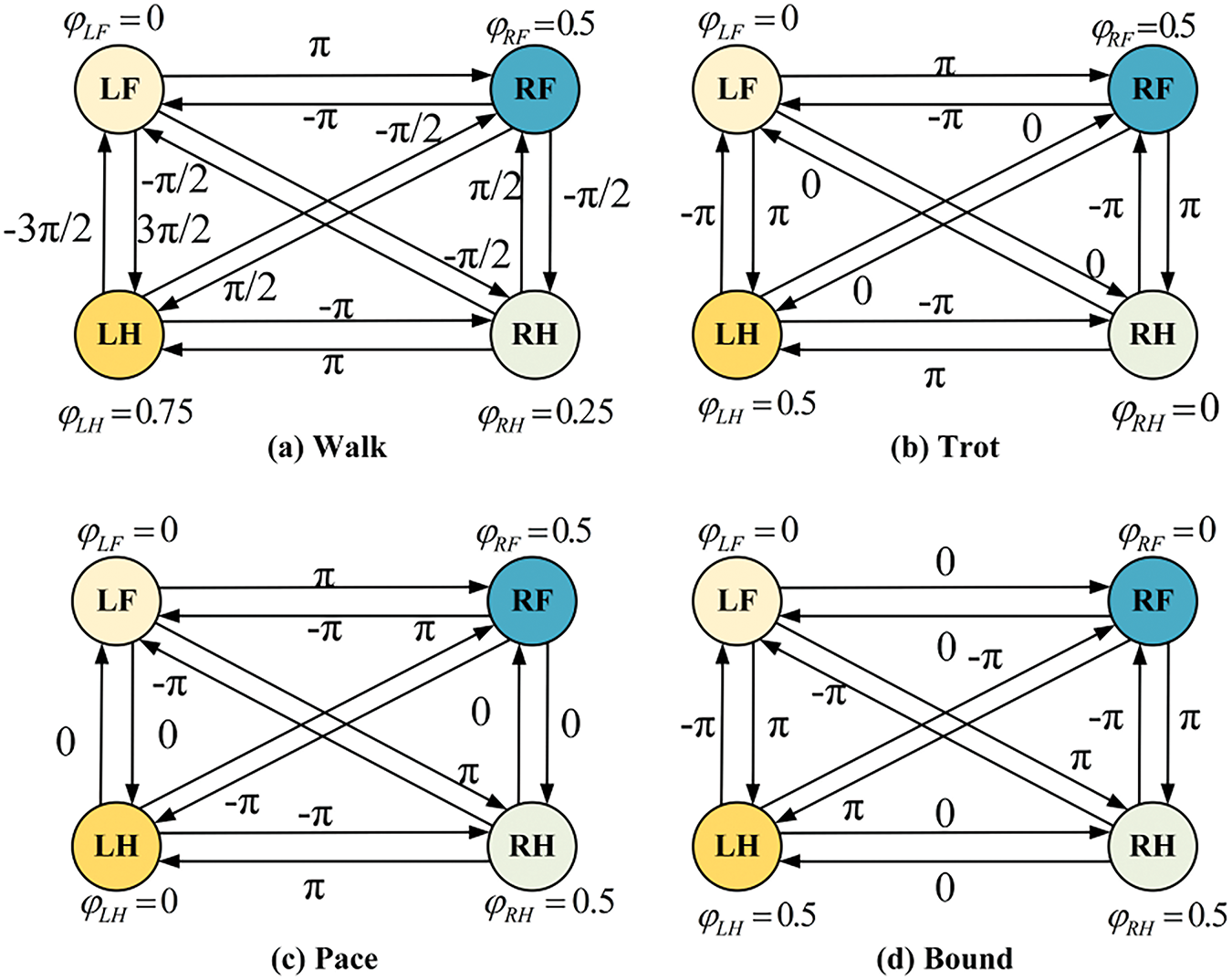
Figure 2: Timing diagram of common gaits
The gaits of quadruped robots are generally classified into static and dynamic gaits [47], with Fig. 3 illustrating the classification of these gaits. A gait is considered a static gait if at least two legs are in the support phase at all times. A gait is considered a dynamic gait if, at any point during the movement, the quadruped robot has at most two legs in the support phase [48]. Static gaits [49] include crawl and walk; Crawl: At least three legs are in the support phase at any given time, and the body may use other parts (such as the abdomen) to assist with movement or stability, offering good stability. Walk: All four legs alternate in a set order between swing and support phases, with a four-beat cycle. Dynamic gaits include Trot [50], Pace [51], Gallop [52], Bound [53], and others; Trot [54]: Diagonal pairs of legs form a group, alternating between swing and support phases in a set order, offering relatively good stability. Pace: Also known as a lateral jog, this gait uses two legs on the same side as a group, alternating in a set order between swing and support phases. This gait tends to roll and is suitable for long-legged animals, effectively avoiding collisions between legs on the same side, but with less stability. Gallop: The front and hind legs form a group, alternating between swing and support phases in a set order, with at most three legs in contact with the ground at the same time. This gait may involve complete aerial phases, generating higher impact forces. Bound: In this gait, the torso exhibits noticeable pitching movements, accompanied by larger impact forces during double-foot jumps. Fig. 4 shows the different gaits of quadruped animals during a single-motion cycle.
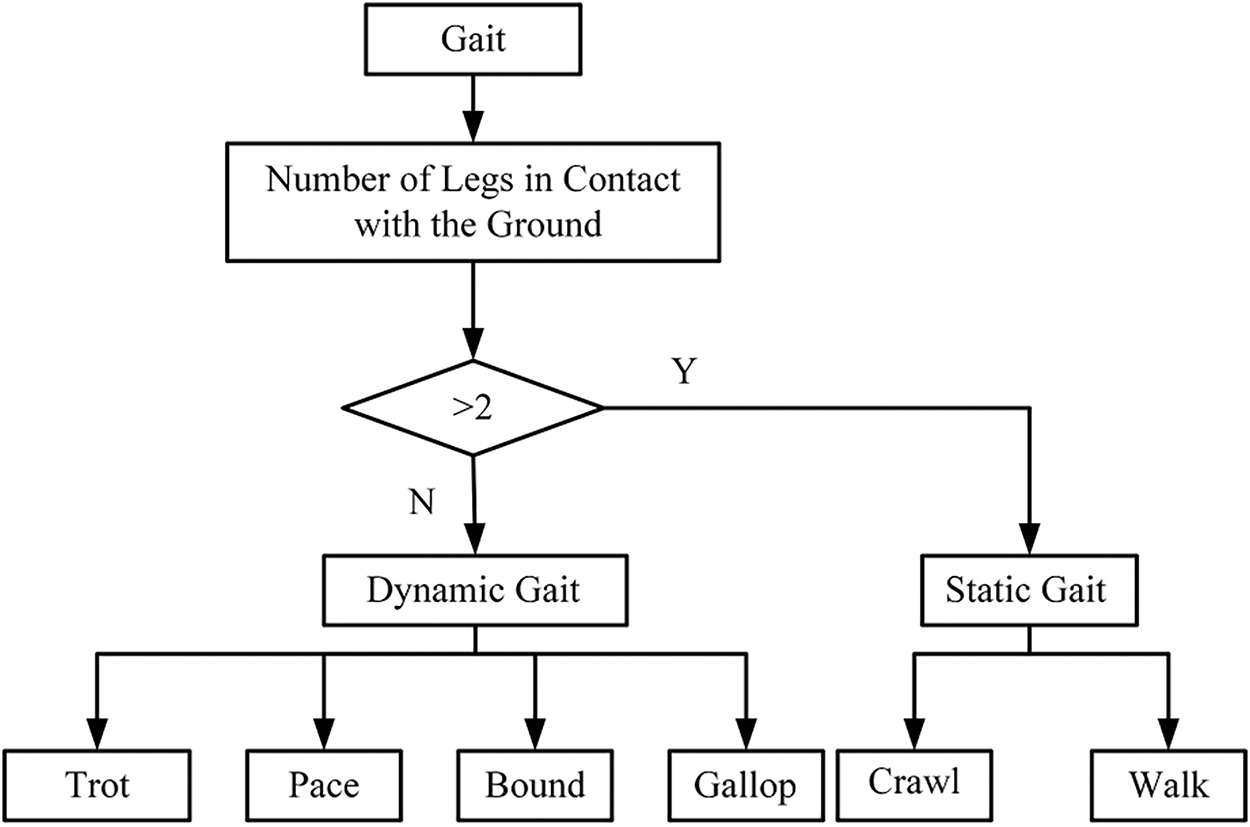
Figure 3: Classification diagram of static and dynamic gaits
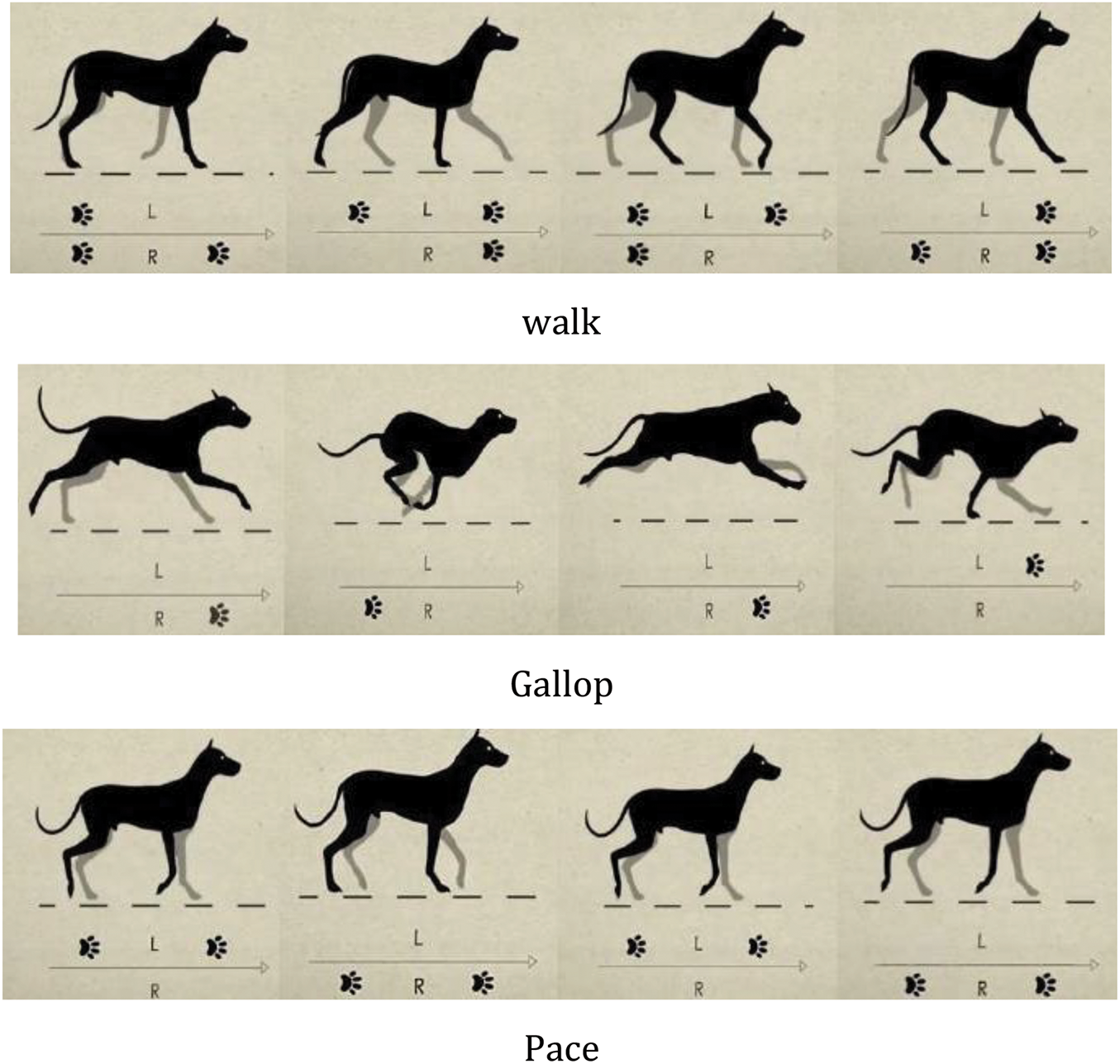
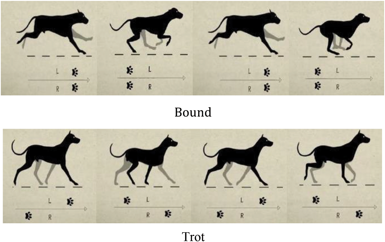
Figure 4: Gait of quadruped animals
2.3 Gait Planning Methods for Quadruped Robots
Currently, gait planning methods for quadruped robots are relatively mature and can be roughly divided into two categories based on the robot’s gait. One category is the planning method for static gaits, with a commonly used approach being gait planning based on ZMP [55] (Zero Moment Point). The other category is the planning method for dynamic gaits, with commonly used approaches including gait planning based on CPG [56] (Central Pattern Generator), gait planning based on SLIP [57] (Spring Loaded Inverted Pendulum), and compound curve trajectory planning [58], among others.
2.3.1 Application of ZMP Method in Gait Stability
ZMP refers to the point where the resultant moment of the ground reaction force, projected onto the horizontal plane, equals zero. It was proposed by the Yugoslav scholar Vukobratovic. ZMP is a commonly used method for analyzing the static gait stability of legged robots [59]. Initially, ZMP was used to analyze the stability of biped robots during motion, and later it was gradually applied to the static stability analysis of quadruped robots. During the robot’s motion, the ZMP must always remain within the support polygon formed by the foot and the ground. This ensures that the robot is in an ideal static equilibrium state. The schematic diagram of the ZMP equivalent position is shown in Fig. 5. When the robot is stationary or moving slowly, the projection of its center of gravity (COG) onto the ground is essentially coincident with the ZMP position [60]. Stability can be determined by whether the projection of the center of gravity is within the support region. However, when the robot moves quickly, due to inertial forces, the positions of the center of gravity and ZMP may shift. In such cases, the robot’s stability can only be determined by the position of the ZMP. Therefore, the ZMP-based gait planning method has significant limitations, as it can only be applied to static gaits and cannot ensure stable control for dynamic gaits.
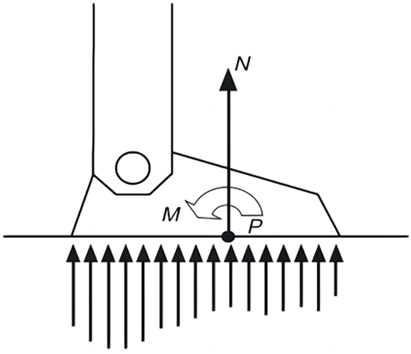
Figure 5: Schematic diagram of ZMP equivalent position
The coordinates of the ZMP are calculated using the resultant of the gravitational and inertial forces and are derived using D’Alembert’s principle [61]. Assuming that the mass of each robot joint link is mi, and the center of mass coordinates of the link are (xi, yi, zi), the resultant of the gravitational and inertial forces is given by:
The resultant moment of the combined force about each coordinate axis is given by:
To move the resultant force from the origin of the reference coordinate system to the ZMP, the components of the resultant force about the X and Y axes at the ZMP must be zero. Therefore:
Therefore, the coordinates of the ZMP are given by:
Since the robot is moving slowly in a static gait, the inertial forces can be reasonably ignored relative to the gravitational force [62]. In this case, the ZMP calculation formula can be simplified to the formula for the center of gravity (COG) position:
When the quadruped robot walks in a static gait, as long as the vertical projection of its COG always remains within the geometric area formed by the three supporting legs, it can be determined that the robot will continue to walk stably. Fig. 6a,b visually demonstrates the principle of this judgment method. By analyzing Fig. 6a,b, and knowing the specific coordinates of legs 2, 3, and 4, and the projection point of the center of gravity, one can easily determine whether the projection point of the center of gravity lies within the polygonal area formed by the supporting feet using mathematical geometric analysis [63]. The specific calculation method is as follows:
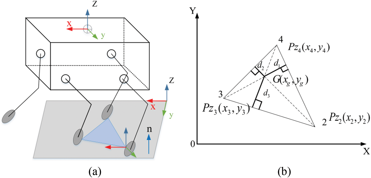
Figure 6: ZMP analysis diagram
Assuming that at a certain moment, the robot’s COG and the contact points have horizontal projections at G(xg, yg) Pz2(x2, y2) Pz3(x3, y3) Pz4(x4, y4) the areas corresponding to ΔPz2Pz4Pz3, ΔGPz2Pz4, ΔGPz4Pz3 and ΔGPz3Pz2 are: SΔPz2Pz4Pz3, SΔGPz2Pz4, SΔGPz4Pz3, SΔGPz3Pz2. By calculating these areas, it can be determined whether the robot’s center of gravity projection is within the support polygon formed by the feet. The specific formulas are as follows:
If the above formula holds, it indicates that the robot satisfies the geometric static stability condition and can achieve stable walking. On the other hand, if the center of gravity projection point lies outside the stable region formed by the supporting feet, it means the robot does not meet the stability condition and is in an unstable state. The indicator used to judge stability is called the stability margin. The stability margin is calculated by determining the minimum distance from the robot’s center of gravity vertical projection point to the edges of the polygon formed by the supporting feet, and this minimum distance is denoted as d. The larger the stability margin d, the more stable the robot is during motion.
Under the condition that the above formula is satisfied, the steps for calculating the stability margin using the polygon static stability judgment method are as follows:
Step 1: Determine the equation of the straight line corresponding to each edge based on the coordinates of the supporting foot points.
Step 2: Use mathematical formulas to calculate the perpendicular distance from the center of gravity projection point to each straight line.
Step 3: Compare all the perpendicular distances and take the smallest value as the stability margin for the current polygon in the static stability analysis.
Given the positions G(xg, yg), Pz2(x2, y2), Pz3(x3, y3), Pz4(x4, y4) the process for calculating the stability margin is as follows:
Step 1: Solve for the equations of lines:
Step 2: Solve for the perpendicular distance of each line:
Step 3: Take the smallest perpendicular distance as the stability margin:
By the above method, the static stability of the quadruped robot can be easily calculated, along with the magnitude of the stability margin that satisfies the stability requirements.
2.3.2 CPG Model-Driven Biomimetic Gait Generation
The exceptional adaptability exhibited in human and animal movement allows them to cope with harsh environments. Modern biological research indicates that such movements, which are regular, periodic, symmetrical, and adjustable under the regulation of the nervous system, are called rhythmic movements. Rhythmic movements are the most common form of movement in humans and animals, with their control core located in the CPG within the spinal cord. CPG is a neural network in the biological spinal cord that can generate regular robotic joint angle and velocity control signals by simulating the structure of lower animal central nervous systems [64]. This structure enables the robot to generate rhythmic motion control signals even when the control and sensor systems are isolated. As a control method that mimics the structure and mechanism of movement control nervous system of higher animals, CPG has been widely applied in robotics. It serves as the “nervous system” of the robot, outputting control signals to regulate the robot’s gait and joint movements. Based on the model construction, CPG models can be divided into two categories. The first category is neuron-based models, which are biologically accurate but are less commonly used due to their complex structure [65]. The second category is nonlinear oscillator-based models, with the Hopf oscillator being the most widely used model due to its simple mathematical form and mature application technology [66]. The oscillatory curves generated by mathematical methods, as inputs for the leg joint positions and velocities, can easily adjust the phase relationships between the robot’s legs. The CPG control method can transmit rhythmic behavior between the neural control system and the physical system, forming a stable limit cycle in the state space, thus giving the robot strong interference resistance [67]. This method not only mimics the basic principles of animal movement control but also provides crucial technical support for robotic motion control.
The specific mathematical model of the Hopf oscillator is as follows:
In the equation, µ is a positive value that determines the amplitude of the oscillator’s output; ω is the frequency of the oscillator; x and y represent the state variables; α is a constant greater than zero, used to control the speed at which the limit cycle converges.
The above equation expresses that the rise and fall times of the Hopf oscillator’s output signal are identical. If this signal is used as the control signal for the robot’s joint angles, it corresponds to the case where the robot’s leg swing time and support time are equal, which is just one special case among various gaits. The gait cycle T represents the time required for a complete movement cycle, i.e., the sum of the leg swing time and the support time. The ratio of the leg support time to the entire gait cycle is called the duty cycle; denoted by β, it is given by:
In real-world environments, robots need to generate multiple gaits to cope with various complex terrains. Therefore, the parameter ω in Eq. (10) is modified as follows:
The gait cycle is:
ωst and ωsw are the frequencies of the stance phase and swing phase of the leg, respectively. The speed at which ω transitions between ωst and ωsw is determined by α.
By adjusting the value of β, the rise and fall times of the oscillator’s output signal can be changed, thereby altering the robot’s leg swing time and support time. This in turn changes the duty cycle [68], allowing the quadruped robot to achieve different gaits.
The CPG control network can be classified into two types based on its connectivity: mesh and chain types. The rhythmic signals generated by this network can be used to regulate the walking motion of organisms. In the absence of higher-level neural commands and external feedback, the CPG neural network can still autonomously generate stable oscillatory signals. This feature is widely applied in quadruped robots, especially for the 8 active joint degrees of freedom involved in the hip and knee joints of their four legs. Typically, there are two common network topologies for control: the first method uses 8 oscillators, with each oscillator corresponding to a joint. This structure employs a hierarchical control network: the first layer contains 4 coupled oscillators that generate control signals for the hip joints; the second layer further generates control signals for the knee joints through unidirectional coupling between the hip and corresponding knee joint oscillators, as shown in Fig. 7. However, due to the larger number of oscillators involved in this structure, the complexity of the CPG control network increases, which in turn raises the difficulty of control [69].
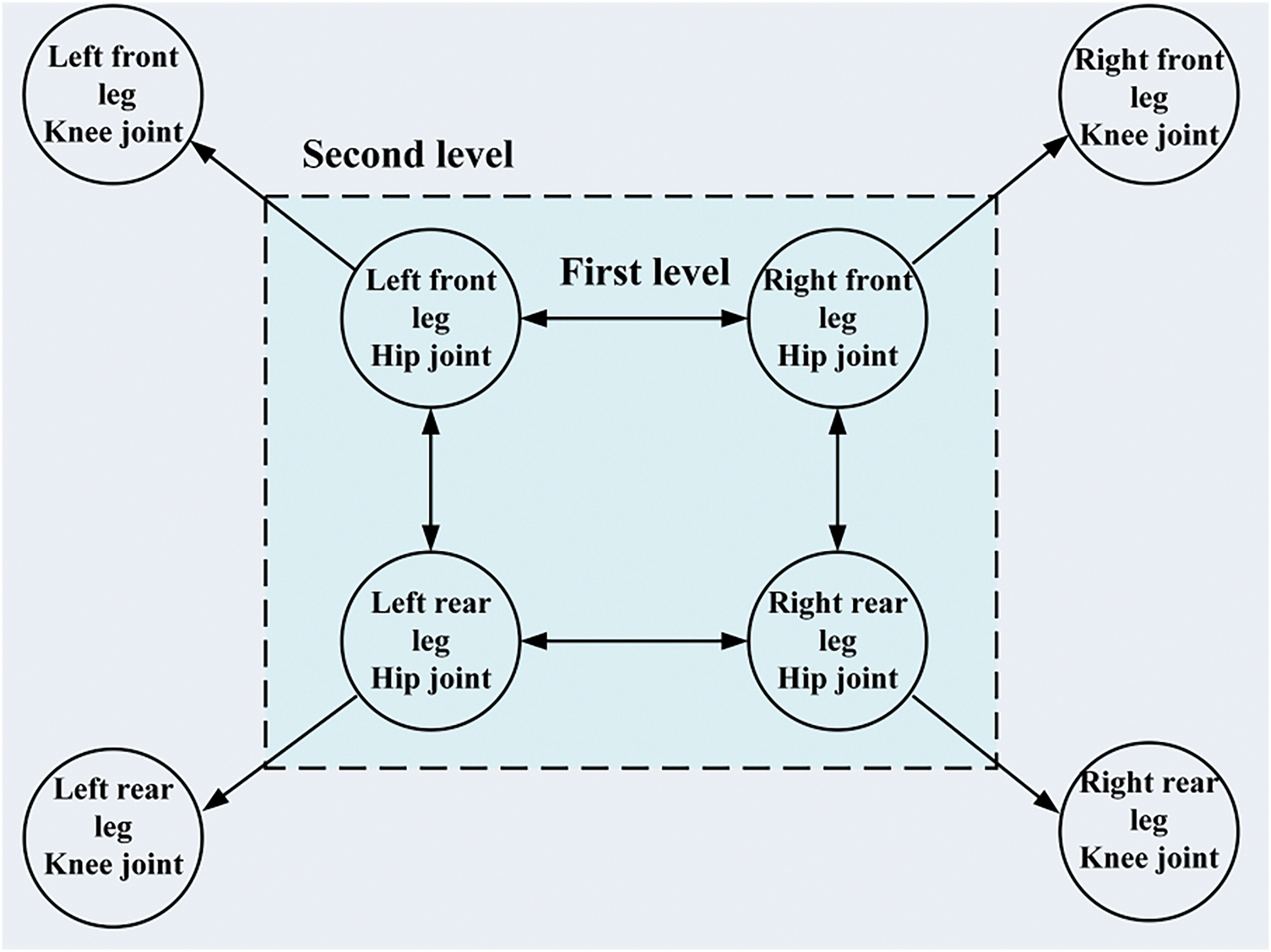
Figure 7: Hierarchical structure of the CPG control network
Another CPG control network, as shown in Fig. 8, requires only 4 oscillators, making the structure simpler. The state variable x output by each oscillator can directly serve as the control signal input for the hip joint, while the state variable y is transformed into the corresponding control signal for the knee joint through a functional relationship. Due to the simplicity of this network structure, the computational complexity is reduced, which shortens the computation time and significantly improves the system’s real-time performance. This CPG control network structure is widely adopted in the gait planning of quadruped robots.
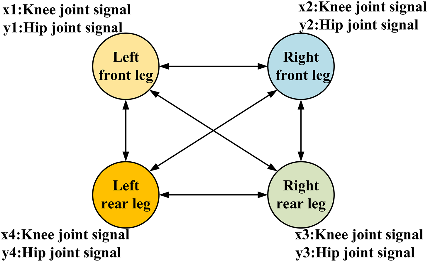
Figure 8: Single-layer CPG control network
By comprehensively analyzing the characteristics of the Hopf oscillator and the single-layer CPG control network, a CPG control network mathematical model was established using 4 Hopf oscillator models to construct the phase coupling relationships [70], as shown in Eq. (14):
θhi: Hip joint control signal; xi: Output of the oscillator;
where
The output pattern of the CPG control network is determined by R. The CPG output signals undergo phase coupling through the connection weight matrix R, ultimately generating 8 output signals with phase relationships, thus achieving different gaits for the quadruped robot.
2.3.3 SLIP Model: Elastic Gait and Energy Optimization
In biological motion, tendons and other energy-storing components reduce impact forces upon landing and enable the storage and reuse of energy. This type of motion is similar to the movement characteristics of the SLIP model. The SLIP model was proposed by Professor Raibert of MIT [71] during the development of a single leg hopping robot. It simplifies the dynamics of a quadruped robot into a single-degree-of-freedom flexible spring and damper model, which allows for dynamic planning using the principles of spring and damping. This helps to analyze the robot’s motion characteristics and control strategies more intuitively. The SLIP model is based on biomimetic principles, as shown in Fig. 9.
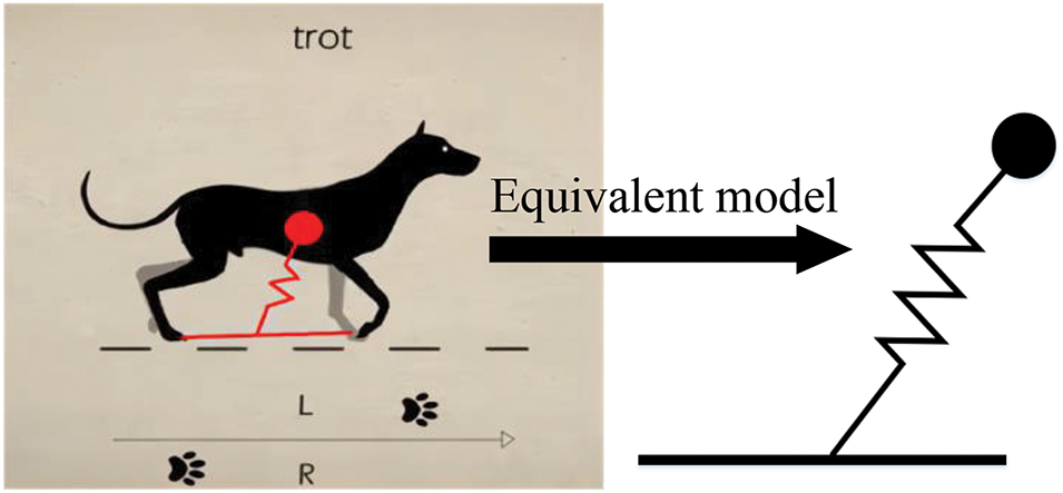
Figure 9: SLIP-based equivalent model of a quadruped animal
In high-speed motion, the contact time of each leg with the ground is significantly shortened, leading to increased impact forces during landing. To maintain stability during high-speed movement, the tendons in the animal’s legs play a key role. They not only effectively absorb the impact energy during landing but also release the stored energy during the push-off phase to optimize movement efficiency and stability. In this respect, springs function similarly to muscles. During one cycle, the compressed spring replenishes energy, while the decompressed spring releases stored energy. The entire movement cycle can be divided into two phases: the stance phase and the airborne phase [72]. In the stance phase, the elastic leg contacts the ground, undergoing natural compression and subsequently decompressing to release energy. In the airborne phase, the spring-loaded leg lifts off the ground, enabling the body to become airborne, as shown in Fig. 10. In subsequent studies, Professor Raibert proposed the “three-part control method” based on this approach, which analyzes the robot’s jumping height, forward velocity, and body posture in three dimensions. This method effectively controls the robot’s movement state during the jumping process. It has had a profound impact on subsequent robotic control research and has driven the development of dynamic motion control. Fig. 11 shows the SLIP model analysis of a quadruped robot.
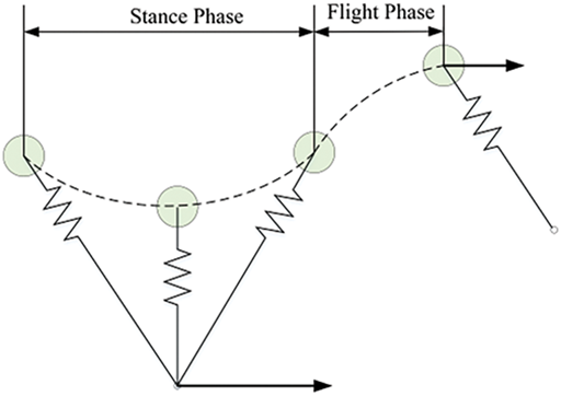
Figure 10: SLIP model
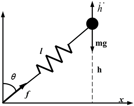
Figure 11: SLIP model analysis of a quadruped robot
The kinematic equations of the SLIP model in three-dimensional space can be decomposed into forward (X direction) and lateral (Y direction) motion components, while in both directions, the Z direction height control is also considered. Specifically, the overall motion can be described as a set of coupled nonlinear differential equations, where the motion in the X and Y directions is influenced by gravity and spring force, while the Z direction is controlled through height control algorithms to achieve both steady-state and dynamic adjustments, ensuring the overall stability and flexibility of the robot. Fig. 10 shows the spring-loaded inverted pendulum model on the ZOX plane. The forward kinematic equations of the SLIP model on the ZOX plane can be expressed by Eq. (18). The analysis method in the ZOY plane follows the same equation.
x0: Initial position in the x-axis direction; z0: Initial position in the z-axis direction. θ: The initial angular displacement of the rotating mass block, which corresponds to the initial pitch angle of the quadruped robot.
During the movement of the quadruped robot, the stance phase and airborne phase alternate to form the robot’s motion characteristics. When the robot’s leg is in the airborne phase, the contact force between the robot’s foot and the ground is Fcontact = 0. In the stance phase, the contact force is Fcontact > 0. A landing event is defined as the transition from the airborne phase to the stance phase, while a take-off event is defined as the transition from the stance phase to the airborne phase.
The airborne phase can be further divided into the ascent and descent phases, based on the sign of the vertical velocity of the robot’s body. Ascent Phase: When the vertical velocity of the body is denoted as
In the support phase, it can be further divided into the compression phase and the recovery phase, based on the trend of the equivalent spring leg length.
Compression Phase: When the virtual spring leg length gradually decreases, the vertical velocity
Assume the equivalent model of the quadruped robot has the following characteristics: the moment of inertia is J, the mass is m, the mass of the equivalent spring leg is ignored, the equivalent spring leg is connected to the model through the center of mass G, with length r, and the spring’s stiffness and damping coefficients are k and c, respectively. The equivalent spring leg has a rotational degree of freedom relative to the center of mass G within the plane, and the rotational angle within the body coordinate system is denoted by
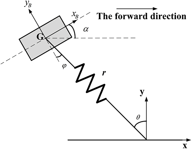
Figure 12: SLIP model dynamics analysis schematic
The system’s kinetic energy is:
The system’s potential energy during the support phase includes both gravitational potential energy and the elastic potential energy of the equivalent spring:
Therefore:
Define the generalized coordinate
To simplify the system, during the support phase, only the spring damping force
The system’s dynamics equation during the support phase is further expressed as:
The result is:
Flight Phase Analysis: When the system is in the flight phase, the entire motion process is only influenced by gravity. The dynamics equation in the global coordinate system is as follows:
Transition Conditions between Flight Phase and Support Phase: The gait cycle of the SLIP model consists of the landing phase and the flight phase, with these two motion states switching periodically. The following are the transition conditions between the two states.
Support Condition: The landing condition occurs when the system is in the flight phase and descending. When the height of the center of mass reaches a critical value, the foot makes contact with the ground, and the system transitions from the flight phase to the support phase. Therefore, the transition condition from the flight phase to the landing phase is:
Flight Condition: When the system is about to lift off, the interaction force between the foot and the ground gradually decreases. At the moment this interaction force reaches zero, the system transitions from the support phase to the flight phase. Therefore, the transition condition from the support phase to the flight phase is:
Fx: The ground reaction force in the x-direction during the support phase. Fy: The ground reaction force in the y-direction during the support phase.
2.3.4 The Smoothing Effect of Composite Curves in Trajectory Optimization
Composite curves generally include cycloidal curves [73], polynomial curves [74], and Bézier curves [75], among which Bézier curves are the most widely used. The cycloidal curve has smooth velocity characteristics and continuous acceleration, but the slope at the start and landing points is too steep, causing the leg to almost become vertical to the ground when lifting or landing, which is inconsistent with the natural gait of legged animals. This leads to increased energy consumption in the robot system. In polynomial curve design, cubic polynomials are simple but discontinuous in acceleration, which causes greater interference between the leg and the body; while quintic polynomials, although smooth in both velocity and acceleration, are more complex and computationally heavier. In comparison, Bézier curves maintain continuity in both velocity and acceleration, and their shape can be flexibly adjusted through control points, making them ideal for foot trajectory planning in complex environments. Reasonable trajectory planning includes the following aspects:
(1) Movement Smoothness: During robot movement, body posture stability must be ensured to avoid sharp vertical fluctuations, lateral swaying, or front-to-back collisions. This requires the gait design to achieve balance in force distribution for each step to ensure smooth center of gravity transfer. Furthermore, the harmony of joint movements is crucial. During leg swinging, the motion of the joints should be smooth, avoiding sharp impacts when lifting or landing the leg. This depends on precise control algorithms to adjust joint movements and achieve smooth and coordinated actions.
(2) Mobility in the Swing Phase: In the swing phase, the robot’s leg should move quickly and efficiently. The foot trajectory should remain smooth, and the joint velocities and accelerations should change continuously without abrupt transitions. This significantly improves walking efficiency and reduces energy consumption [76].
(3) Foot Contact Stability: During walking, the robot’s foot must maintain firm contact with the ground, avoiding slipping or dragging. This requires the foot design to adapt to various ground conditions, while the control strategy ensures foot stability during ground contact.
The origin of Bézier curves can be traced back to 1959 when Paul de Casteljau used numerical methods to plot Bézier curves in his algorithmic research. Later, the French engineer Pierre Bézier successfully applied this curve to automotive body design. Due to its excellent controllability and smoothness, Bézier curves quickly found widespread applications in various fields [77]. The mathematical expression of a Bézier curve is as follows:
Considering the computational complexity and the practical requirements of the task, a cubic Bézier curve is chosen as the trajectory curve for the foot end. The height of the swinging leg is considered as the highest point of the curve. The trajectory curve of the foot end is divided into the ascending trajectory and descending trajectory, with the position curve in the Z-axis direction given by Eq. (30) as follows:
P0 represents the initial position of the foot end; Pf is the landing position; h denotes the swing leg’s lift height; and t is the ratio of elapsed swing time to the total swing phase duration. For the trajectories along the X and Y axes, since there are no intermediate point constraints, the trajectories are not divided into ascending and descending phases. Therefore, the curve expression is as follows:
By substituting the actual coordinates [x,y,z] of P0 and Pf, as well as the leg-lift height h, the foot-end trajectory can be derived. Taking the 2nd and 4th-order Bézier curves as examples, the expressions are shown in Eq. (32). The resulting curve approximates the triangular area defined by the starting point P0, control point P1, and endpoint P2, as illustrated in Fig. 13.
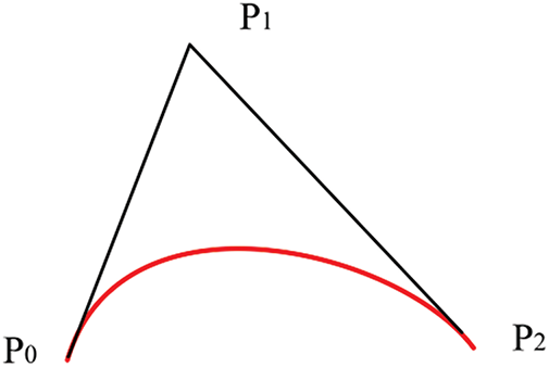
Figure 13: 2nd-order Bézier curve fitting
Eq. (33) represents the 4th-order Bézier curve. The shape of the curve changes and adapts based on the number and position of control points, as shown in Fig. 14.
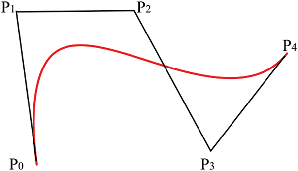
Figure 14: 4th-order Bézier curve fitting
Bézier curves exhibit strong shape controllability, and their higher-order derivatives also remain Bézier curves. This ensures smooth transitions in the trajectory, meeting the requirements of an ideal path. As a result, Bézier curves are widely used in foot trajectory planning for quadruped robots.
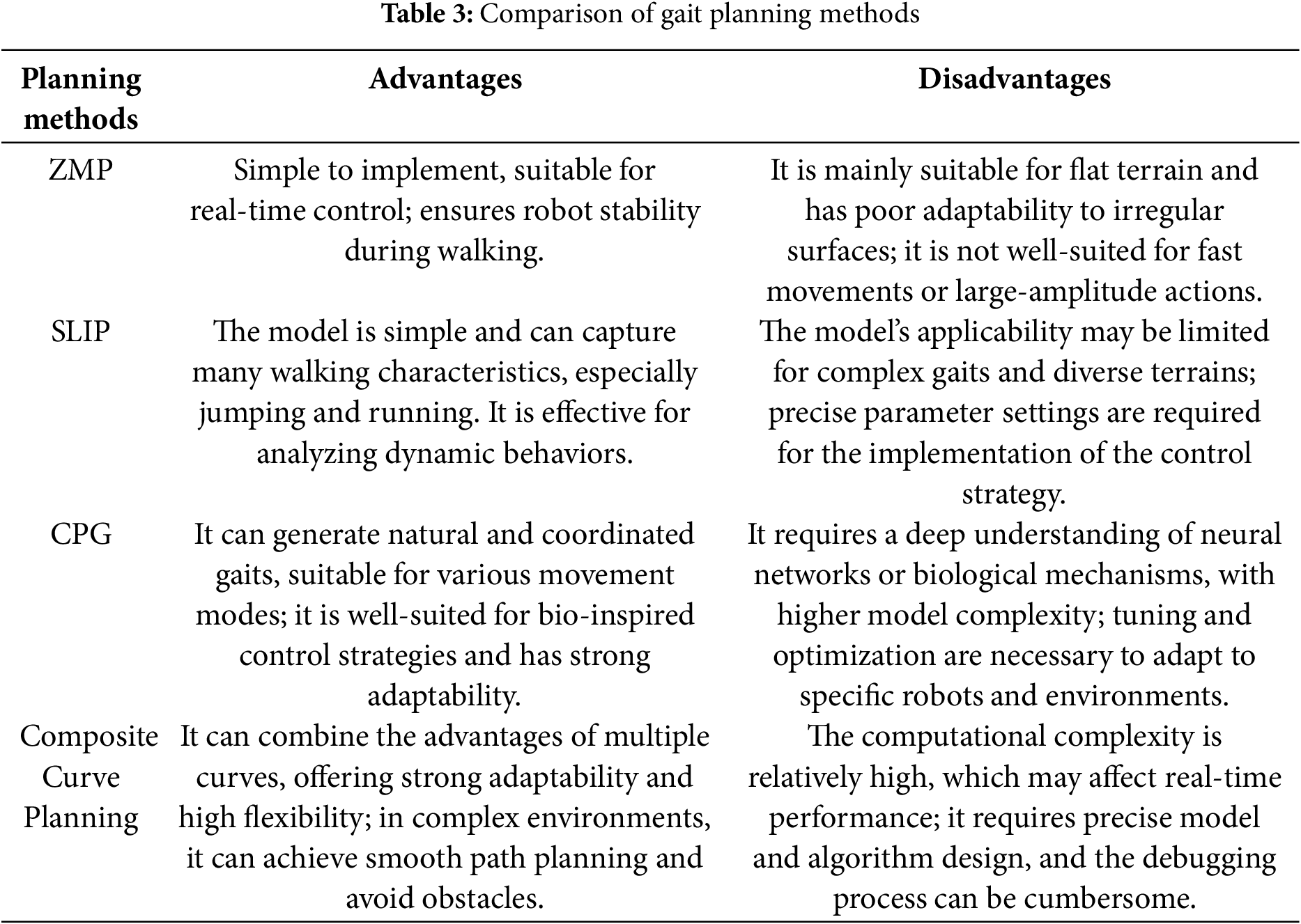
The choice of different gait planning methods should be comprehensively considered based on the specific application requirements, environmental complexity, and the dynamic characteristics of the robot [78]. For most robotic applications, it is often necessary to combine multiple methods to achieve optimal results. Table 3 provides a comparison of various gait planning methods.
3 Motion Control of Quadruped Robots on Multiple Terrains
Motion control of robots [79] refers to the use of algorithms during the robot’s movement to control the torque of its joints. It is employed to manage various states of the robot, including speed, posture, and stability while minimizing impact forces during contact with the ground. This enables dynamic stability and robustness. In the field of robotics, motion control for multi-legged robots has always been a key focus and a challenging research area. Currently, motion control methods for quadruped robots [80] mainly include model-based control methods, reinforcement learning-based control methods, decentralized control strategies, distributed control strategies, and hybrid control algorithms.
3.1 Model-Based Control Methods
Model-based control methods, as a classical approach, are widely applied in the field of legged robots. This method first simplifies the robot’s mechanical structure and then performs kinematic modeling based on its physical parameters. By analyzing and deriving the relationship equations between the foot trajectory and joint angles or the forces at the joints, the desired joint values or forces can be determined based on the expected motion. This is a widely applied and classic motion control method for quadruped robots. Currently, representative control methods include: MPC [81] (Model Predictive Control), VMC [82] (Virtual Model Control), WBC [83] (Whole-Body Control), and others.
3.1.1 Optimal Control: The Advantages of MPC in Dynamic Control
MPC is a model-based motion control method that emerged in the 1970s [84,85] and has become one of the most commonly used control strategies in robotics in recent years. It is an efficient control strategy that predicts the future state changes of the system by constructing a predictive model of the robot, transforming the control problem into a constrained optimization problem. In each control cycle, MPC calculates a series of control inputs based on the current state, aiming to minimize the deviation from the target trajectory while satisfying the system’s actual constraints. Fig. 15 illustrates the principle of MPC. Specifically, MPC uses sensor data to obtain the state information at each sampling time, solves the optimization problem over a finite time horizon, and sends the resulting action sequence to the robot. The process is repeated at each sampling time, with the control strategy being updated in real-time to adapt to the system’s dynamic changes. Fig. 16 shows the MPC control flow for a quadruped robot.
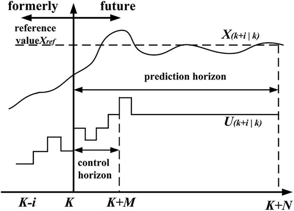
Figure 15: Schematic of MPC
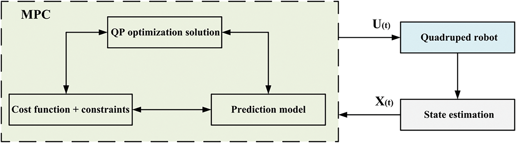
Figure 16: MPC control flowchart for quadruped robot
MPC generally consists of three stages: building the predictive model, online rolling optimization, and feedback correction.
Building the predictive model: This is the core of MPC. Its main function is to link the historical information of the robot system with future inputs, describing the robot’s dynamic behavior, and enabling the prediction of the system’s future output.
Online rolling optimization: MPC takes the first optimal solution from the series of optimal solutions as the current control input. Unlike traditional optimal control algorithms that perform offline optimization, MPC adopts a real-time rolling optimization process [86], thereby improving control performance.
Feedback correction: MPC can handle issues such as external environmental disturbances or model mismatches. In a new sampling cycle, MPC compares the actual system output with the theoretical value, adjusts the results of the predictive model, and then recalculates the optimal control solution.
At time k, the system state is x(k), and the system uses past input information to predict its future output state.
Select a performance index for online optimization calculation to obtain the optimal control input sequence u*(k) = [u*(k∣k), u*(k + 1∣k), …, u*(k + N−1∣k)] within the prediction time horizon N.
The first term of u*(k), u*(k∣k), is taken as the input control at time k.
At time k + 1, repeat the above steps in the new time domain.
MPC uses the state variables X(t) at time k and the pre-established prediction model, considering the constraints, to solve a series of optimal control values over the time domain using QP (Quadratic Programming) optimization [87]. The first optimal control value is then applied to the current time step U(t).
In quadruped robot motion control, MPC can accurately describe the system dynamics and predict future states, making it a commonly used control strategy. Through rolling optimization, MPC can calculate the optimal control inputs in real-time while satisfying various constraints, enabling efficient management of the robot’s motion and precise trajectory tracking [88]. The MPC control block diagram is shown in Fig. 17. The following section will provide a detailed description of the specific control process of MPC for quadruped robots.
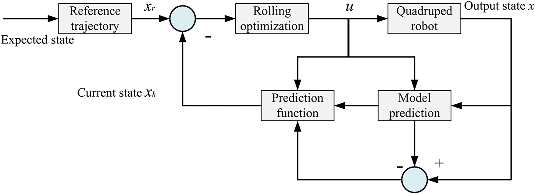
Figure 17: MPC control block diagram
Modeling: Based on the dynamic characteristics of the quadruped robot, establish an appropriate discrete-time model (e.g., a rigid body dynamics model), defining the state variables
xref: Desired state Q, R: Weight matrices used to balance the errors.
Constraints:
Dynamic constraints: Ensure that the state changes within the prediction horizon conform to the system’s dynamic equations.
Input constraints: Set physical limits on control inputs (e.g., foot forces or joint angles).
State constraints: Ensure that the robot’s foot trajectory and center of mass position remain within feasible bounds.
Rolling optimization:
Prediction phase: Based on the current state xk, use the model to predict the system behavior over the next N time steps. Optimize the cost function J and compute the control input sequence uk: k+N−1.
Execution phase: Only use the first step of the optimized result
Feedback update: Use data collected from sensors to measure the actual robot state and update xk, perform rolling prediction, and repeat the above process to form a closed-loop control.
The core of MPC lies in transforming the control problem into an optimization problem within a finite time window. By considering future constraints and objectives, and utilizing continuous prediction and optimization, it provides proactive and adaptive control capabilities for the system’s dynamic behavior.
3.1.2 VMC: Real-Time Motion Control and Stability Assurance
VMC was proposed by Jerry Pratter at the Massachusetts Institute of Technology in the 1990s [89] and was successfully applied to biped robots [90]. The core principle of VMC is the introduction of non-existent virtual components, through which a connection is established between the points of force application in the mechanism and the external environment. By calculating the virtual forces and torques acting on these virtual components, the robot can achieve the desired motion goals. Next, the Jacobian matrix is used to map these virtual forces to the desired joint torques of the robot, which are then used as inputs to control joint motion, resulting in effective control outcomes. VMC is a variant of compliant impedance control [91] (compliant impedance control can be classified as a model-based motion control method, but unlike traditional model-based control, compliant control focuses more on the robot’s ability to perceive and adapt to both its body and the environment during control. It emphasizes dynamic interaction between the controller and the external environment, improving the robot’s control performance and adaptability). The equivalent model of VMC for quadruped robots is shown in Fig. 18. Virtual model control reflects the force interaction characteristics between the robot and the external environment more simply and directly. It is important to note that in virtual model control, the virtual force [92] acts on imaginary virtual components that do not physically exist and do not correspond to any physical mechanism. The virtual force is actually the resultant force acting on the robot’s foot, which is achieved through joint drives during actual motion. There is a mapping relationship between the foot forces and joint torques, determined by the robot’s mechanical structure. By using the robot’s forward kinematic model, position information of the foot relative to the robot’s leg-side swing joint coordinate system can be obtained, thereby determining the mapping relationship between the foot workspace and the joint space:
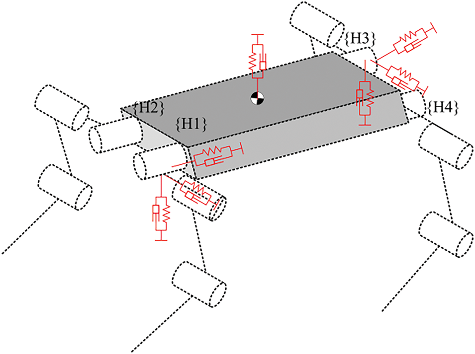
Figure 18: Equivalent model of VMC for quadruped robot
Find the partial derivative of x concerning q:
That is:
The principle of virtual work:
The J matrix changes as the robot’s joint angles q vary.
The virtual model control method is intuitive and simple, not relying on precise dynamic modeling. Although it cannot achieve high-precision position or force control, it focuses more on perceiving and responding to external disturbances in practical applications, rather than strict trajectory constraints. Compared to workspace control, its accuracy is lower, but it is sufficient to meet the requirements for foot height and trajectory when a legged robot is walking or running, where precision is not critical. Virtual model control simplifies complex motion models, converting high-level posture commands into torque control for the leg joints, intuitively reflecting the robot’s motion state, effectively interacting with the environment, and ensuring stability. When controlling a quadruped robot, spring and damping components are used as virtual elements for control. The basic formula for calculating virtual forces is as follows:
Fvmc: The virtual force generated by virtual components; Kvmc: Spring constant; Dvmc: Damping coefficient; xd: Desired displacement. x: Actual displacement;
By using the force Jacobian matrix to map the end-effector virtual force to the joint space, the leg’s adaptation to the body motion can be achieved. Fig. 19 shows the virtual model control block diagram.
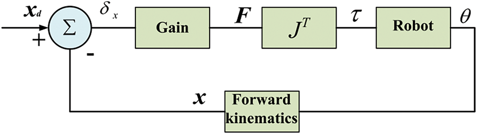
Figure 19: Virtual model control block diagram
Due to the characteristics of virtual model control, a certain control error is inevitably generated during the motion control of a quadruped robot. The desired joint torques calculated are based on a simplified robot model, but in practical applications, complex factors such as system inertia, centrifugal forces, and structural friction must also be considered. These factors may cause discrepancies between the actual motion and the ideal motion. By properly adjusting the damping and stiffness coefficients in the control model, this difference can be effectively reduced, bringing the motion state closer to the target. Virtual model control is one of the easiest force control methods to implement in practice, as it does not require considering the robot’s complex dynamic relationships and can achieve good force control characteristics with minimal computational effort. The algorithm’s intuitiveness and simplicity have led to its widespread use in the motion control field of quadruped robots [93].
3.1.3 Motion Control Based on WBC: Multi-Task Coordination and Dynamic Balance
To address the issue of redundant motion coordination in robot systems, Khatib et al. first proposed a task-oriented whole-body dynamic coordination control framework in 1987 [94], which is the prototype of WBC. In 2004, Khatib applied this method to humanoid robot control [95] and formally named it Whole-body Control (WBC).
When a quadruped robot is viewed as a multi-body system with a floating base, the focus of research is on determining the position and posture of the robot’s base and legs. Its state variables include the body configuration and leg joint angles. The control forces within the system consist of joint torques and ground reaction forces. The desired trajectories of the body and legs can be generated through preset planning or constraints [96]. In such systems, in addition to constraints related to contact and friction with the ground, tasks can be represented as equations or inequality constraints involving state variables or joint torques. To resolve task constraint conflicts, appropriate optimization equations must be used in the design of hierarchical control [97]. This hierarchical controller is called the whole-body controller (WBC), which can be roughly divided into two types: WBC based on Null Space Projection (NSP) [98] and WBC based on Hierarchical Quadratic Programming (HQP) [99].
NSP-based WBC: The NSP method emerged earlier, and its basic idea is to map low-priority tasks into the null space of high-priority tasks to ensure that low-priority tasks do not interfere with the execution of high-priority tasks. The task space vector and the joint space vector satisfy the kinematic constraints:
Taking the derivative of Eq. (39) gives:
When the dimension of joint space N is greater than the dimension of task space M, the task has redundant degrees of freedom. For tasks with redundant degrees of freedom, the Jacobian matrix J(q) has a right inverse J+ and satisfies JJ+ = I. When the Jacobian matrix is full rank, the right inverse J+ is given by:
The mapping from task space velocity to joint space velocity is represented as:
If the task has redundant degrees of freedom, there will be a null space. In the case of a robot, it refers to the set of all joint space velocities that result in a zero-task space velocity.
The null space projection matrix N can project any joint velocity onto the corresponding null space projection matrix.
Null space projection matrix N: I−J+J; and it satisfies the properties: N+ = N, NN = N
If there are two tasks,
Therefore,
Therefore, for task
Based on the above theory, a multi-task priority control strategy in the null space can be derived. For ni tasks, the joint space velocity that satisfies the task priorities is:
Based on HQP WBC: Tasks are represented as constrained optimization problems, with slack variables introduced to address infeasible constraints. Hierarchical Quadratic Programming, as a cascade form of quadratic programming, can be used to solve multi-task problems with priorities.
Rewrite Eq. (43) in the optimized form:
When considering only
S1: The slack variable for task T1.
Task T is defined as a set of linear equality or inequality constraints on the solution vector
When solving a set of tasks T1, ..., Tp simultaneously, they can be either weighted relative to each other or solved strictly according to priority order; for example, solving in strict priority order based on the null space:
Once the optimal solution x* for p tasks is obtained, to ensure strict priority separation, the next solution xp+1 is found in the null space
Let
where:
The above expression represents the hierarchical QP form based on the null space. By solving this hierarchical QP problem [100], the desired state variables x* can be obtained, which include the robot’s velocity, acceleration, and contact forces, among other information. This information is then integrated with the robot’s dynamic model to compute the required joint torques and pass it to the controller. In this way, control of multi-task problems with priorities can be achieved, enabling trajectory tracking in the joint space and thereby completing tasks planned in the task space.
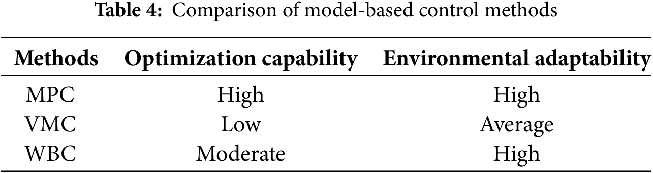
Model-based control methods can be categorized into multiple levels of complexity. Virtual Model Control (VMC) is an intuitive and highly real-time approach, suitable for achieving simple gait control. Whole-Body Control (WBC) optimizes global dynamic objectives and finds broad applications in multi-task control. Meanwhile, Model Predictive Control (MPC) represents a more advanced optimization-based control method, featuring online rolling optimization capabilities that enable gait trajectory and energy consumption optimization in complex environments. The applicability and advantages of these methods lie in balancing real-time performance, computational resources, and adaptability. Different application scenarios call for selecting the appropriate control method, as illustrated in Table 4.
3.2 Autonomous Learning-Based Control Methods
Autonomous learning-based control methods mainly rely on Deep Reinforcement Learning (DRL) algorithms [101]. With the rapid development of artificial intelligence and computer science technologies, DRL has shown great potential in the motion control of legged robots. In recent years, the development of deep learning has propelled reinforcement learning to new heights. The combination of deep learning and reinforcement learning enables the handling of high-dimensional, continuous action and state spaces [102]; reinforcement learning learns better control strategies through continuous trial and error, exhibiting strong decision-making capabilities [103]; while deep learning has strong perceptual abilities [104]. Therefore, the integration of these two, DRL, breaks the traditional constraints in the field of robotics. It demonstrates enormous potential in the field of robotics, as DRL does not require extensive computation or precise parameter design. The robot learns motion strategies through interaction with the environment, possessing the ability for autonomous learning, making it more adaptive and versatile [105]. The use of DRL for motion control in robots is becoming a hot topic in the research of quadruped robots.
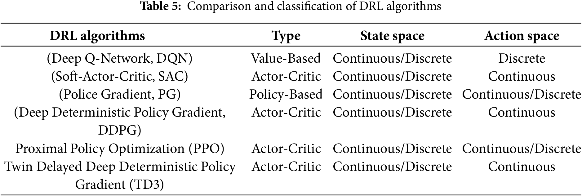
DRL is an end-to-end learning method with strong generalization ability [106]. Based on the type of update strategy, DRL is divided into three categories: Value-Based [107], Policy-Based [108], and Actor-Critic [109], as shown in Table 5. The learning process of DRL can be described as follows:
① Initialize the network parameters for both deep learning and reinforcement learning;
② The agent observes the environmental data through its perception system, where deep learning processes the high-dimensional environmental perception data, which includes specific feature state representations;
③ The decision-making system evaluates the value function of each action based on expected rewards and uses the policy network to map the current state to the output action;
④ The action reacts to the environment and results in a new set of observations. This process repeats steps ②–④ in a loop.
Value-Based Algorithm (DQN): The agent’s state space and action space are used as inputs, and the expected cumulative reward over time is output. Based on this expectation, the action with the highest value in the action space is selected. This type of algorithm requires traversal of all action values, so the action space must be discretized. The loss function of the DQN [110] algorithm is as follows:
θNN: Neural network weight parameters. Q(st+1,a,θNN): Q-value obtained by the neural network with parameters θNN; r: Reward value; γ: Discount factor.
The squared error between the actual Q-value and the estimated Q-value is used as the loss function. Gradient descent is employed to update the network parameters, resulting in the final converged value.
Policy-Based Deep Reinforcement Learning Algorithms: The current policy is used to obtain the corresponding action space in the state space. Unlike Value-Based methods, Policy-Based methods do not use a value function, but instead evaluate the effectiveness of the policy by executing it multiple times [111]. The update process calculates the gradient of the network parameters (such as the weights and biases of the neural network) based on the obtained rewards, adjusting the learning parameters in the direction that increases the reward, thereby updating the policy. Policy-based deep reinforcement learning algorithms update parameters in an episodic manner, but they suffer from lower learning efficiency and higher convergence difficulty.
Actor-Critic Algorithm: This improves the episodic update method in Policy-Based approaches [112] by adopting a single-step update mode from Value-Based algorithms while combining the policy gradient from Policy-Based methods. In this approach, the Actor-network takes the state space as input and outputs the corresponding action space, while the Critic network takes both the state space and the action space output by the Actor as input to evaluate the value of the action. By comparing the actual reward with the value estimate of the Critic, an error can be calculated. The Critic network uses the time difference (TD) error obtained after the agent’s single-step execution as the loss function and updates the Critic network parameters intending to minimize this loss. Meanwhile, the Actor-network updates its network parameters based on the TD error provided by the Critic.
Currently, commonly used deep reinforcement learning methods in legged robot control include DDPG and PPO.
3.2.1 Deep Deterministic Policy Gradient (DDPG)
DDPG adopts the Actor-Critic (AC) framework [113], combining the advantages of both policy gradient and value function methods. It is a deep reinforcement learning algorithm designed to solve continuous action control problems, which not only enhances the stability of learning but also improves convergence. It uses an experience replay strategy by storing samples in an experienced pool and sampling them with a normal distribution to break the correlation between samples, thereby accelerating training speed [114]. This method effectively balances the exploration of unknown environments with the exploitation of the old policy, enabling precise and effective control of quadruped robots. Table 6 provides the pseudocode for the DDPG algorithm [115], and its flowchart is shown in Fig. 20.
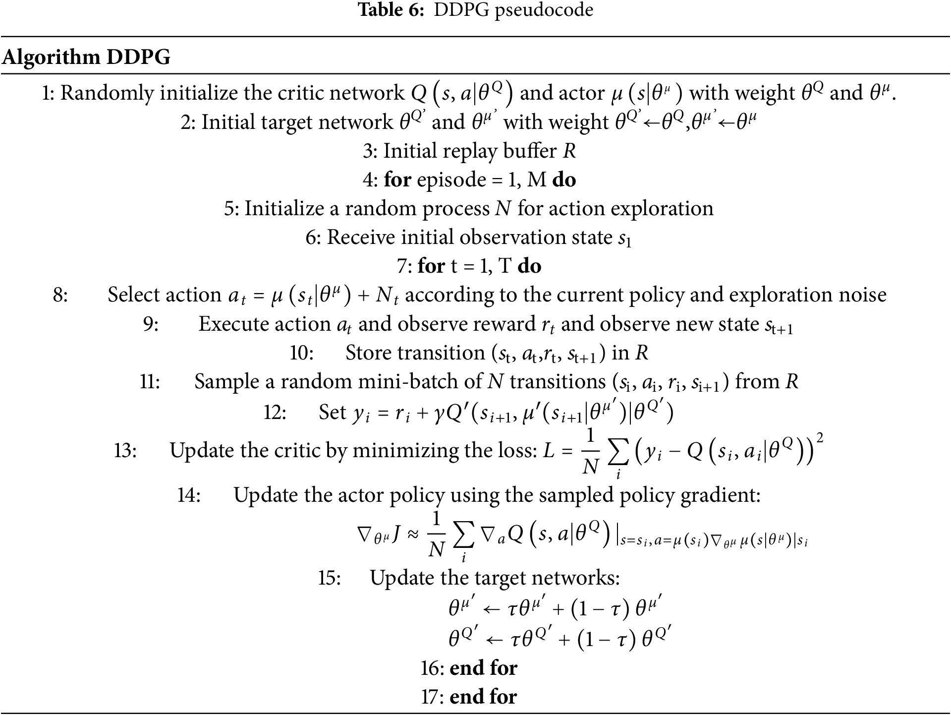
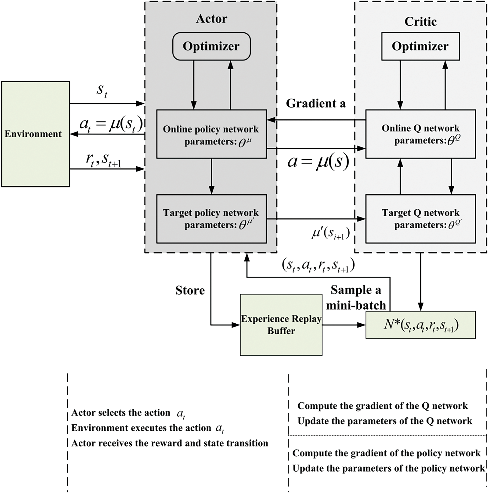
Figure 20: DDPG algorithm flowchart
{\leftskip0pt\rightskip0pt plus1fill}p{#1}}?> {\leftskip0pt plus1fill\rightskip0pt plus1fill}p{#1}}?>Online Actor-network: Represents the action policy
Target Critic network: Represents the action policy
Online Critic network: Represents the value function
Target Critic network: This network has an evaluation function, used to estimate the action chosen in the new state and calculate the optimal action
3.2.2 PPO’s Policy Optimization and Efficient Decision-Making Capability
PPO algorithm is an important deep reinforcement learning method [116], based on the idea of natural gradients, aiming to improve training stability and convergence speed. PPO limits the step size of policy updates to prevent instability caused by excessively large updates. Its core method [117] introduces a clipping mechanism or Kullback-Leibler divergence penalty in the objective function to ensure that the deviation between the new and old policies remains within a reasonable range. This approach not only retains the improvement of the advantageous policy but also avoids the training instability caused by large policy jumps. In practical applications, such as robot control, the PPO-Clip method is particularly common [118]. Table 7 presents the pseudocode for the PPO-Clip algorithm [119], and the algorithm flowchart is shown in Fig. 21.
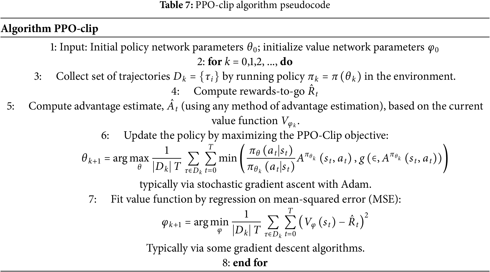
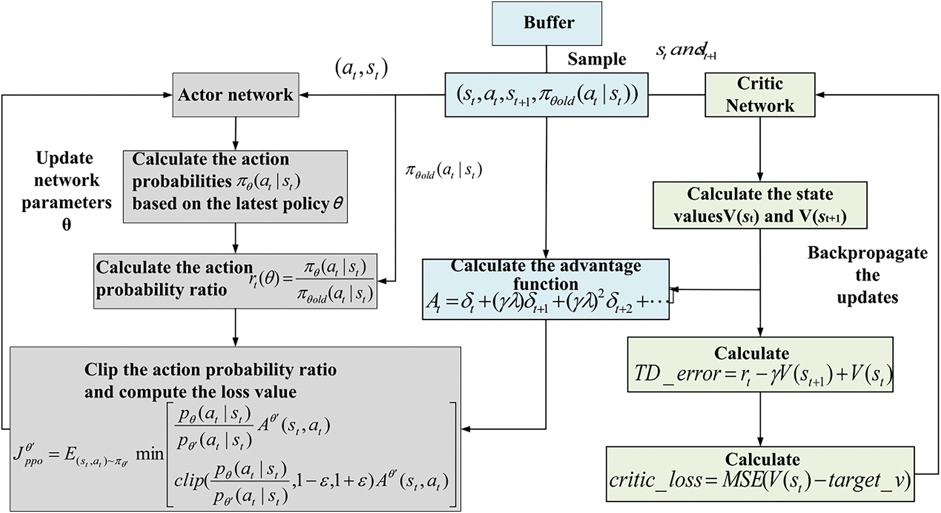
Figure 21: PPO-clip algorithm flowchart
{\leftskip0pt\rightskip0pt plus1fill}p{#1}}?> {\leftskip0pt plus1fill\rightskip0pt plus1fill}p{#1}}?>γ: Discount factors, used to balance the weight between short-term and long-term rewards. λ: GAE weight parameter, used to control the trade-off between bias and variance. δt: TD error, calculated as:
In practical applications, due to the inconvenience of infinite summation, GAE uses a finite horizon T to truncate the estimation, meaning it only computes the advantage values within a finite number of steps.
GAE finds the right balance between bias and variance depending on the value of λ. When λ is closer to 1, the estimation becomes smoother, but the variance is larger. When λ is closer to 0, it focuses more on the current reward, resulting in a smaller variance but larger bias.
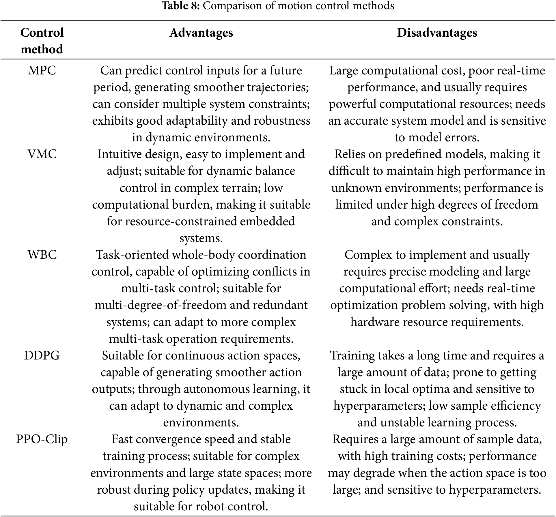
The advantages and disadvantages of several commonly used motion control methods for quadruped robots are shown in Table 8. This table summarizes the pros and cons of each control method in the application, allowing for the selection of the most suitable control method based on specific task requirements and hardware conditions.
3.3 Decentralized Control Strategies and Distributed Control Strategies
Decentralized control refers to a system in which no central controller coordinates the overall behavior [120]. Instead, each component of the systems such as the joints or actuation modules of the robot—operates and makes decisions independently. Each component typically completes tasks based on local perception information (e.g., sensor data) and its localized objectives [121]. The primary goal of this control method is to achieve efficient system operation by eliminating the reliance on centralized control strategies. In contrast, distributed control involves multiple control modules within the system that can operate independently [122] while collaborating through mechanisms such as information sharing or local coordination to achieve complex tasks. Unlike decentralized control, distributed control typically incorporates a form of local information exchange and coordination mechanism [123]. When making localized decisions, each module may need to access state information from other modules to adjust its actions in alignment with global objectives.
3.3.1 Decentralized Control Strategies
In quadruped robot motion control, decentralized control involves distributing control tasks across multiple independent control units. These units do not rely on global information but instead use their local data to execute motion control. Each control unit operates autonomously, managing its motion without requiring input from other units [124]. The main strategies include:
a: Local Feedback Control
Each leg control unit utilizes local sensor data (e.g., joint angles, velocities, accelerations) to independently perform feedback adjustments. Using local feedback controllers, such as Proportional-Integral-Derivative or Linear Quadratic Regulator controllers, each leg can achieve independent control of position, velocity, or force [125]. During specific gaits, the control units of individual legs adjust independently based on their local feedback (e.g., joint angle or velocity errors), ensuring precise movement. This method simplifies the control of architecture and reduces computational complexity. Since each leg can function autonomously, it offers high flexibility, making it well-suited for dynamically changing environments.
b: Feedforward Control
Feedforward control calculates the required control input in advance using the system model or predefined trajectory information, without relying on feedback error adjustments. This approach effectively prevents system deviations during motion [126]. In quadruped robot locomotion, feedforward control can predict the trajectory of each leg and preemptively correct deviations by applying pre-calculated control inputs. Particularly in scenarios involving rapid motion or complex gaits, feedforward control significantly reduces delays and errors. By anticipating control inputs, it not only shortens response times but also enhances the precision of the control system.
c: Adaptive Control
Adaptive control enables each control unit to automatically adjust its parameters in response to changes in the environment or the robot’s dynamic state [127]. This method is especially suitable for scenarios where the system’s dynamic characteristics are uncertain. For instance, when a quadruped robot traverses uneven terrain, the controller for each leg can dynamically adapt its control parameters based on ground conditions, such as friction coefficients or slopes. This ensures the robot maintains stable locomotion across various terrains. Adaptive control effectively handles system uncertainties and external disturbances, offering flexibility to accommodate diverse environmental demands.
3.3.2 Distributed Control Strategies
Distributed Control achieves global objectives through information exchange and collaboration among multiple control units (e.g., the four legs of a quadruped robot) [128]. Unlike decentralized control, distributed control relies on communication and coordination between control units to ensure the successful accomplishment of global goals. The primary control strategies include:
a: Distributed Model Predictive Control (DMPC)
Each control unit (e.g., the controller for each leg) utilizes a local model for prediction and optimization while coordinating through information exchange to achieve global control objectives. DMPC optimizes current control inputs by predicting future states for each control unit [129]. In complex gait tasks such as jumping or stair climbing, DMPC allows the controllers of each leg to dynamically adjust their trajectories based on the predictive information of the other legs. For instance, during a jumping motion, each leg’s control unit predicts future forces and positions to optimize its motion control. By facilitating information exchange and collaborative optimization among multiple control units, DMPC significantly enhances global performance, mitigating the impact of local optimizations on overall stability.
b: Cooperative Control
In cooperative control, each leg of the quadruped robot works collaboratively to optimize global objectives. Each control unit not only relies on its sensor data but also shares information with other control units to jointly accomplish tasks [130].
For instance, during gait coordination, the control unit of each leg dynamically adjusts its actions based on information from other legs, ensuring coordinated and balanced overall motion. This approach significantly enhances the system’s robustness and coordination, facilitating efficient collaboration among multiple control units to achieve stable global behavior.
c: Multi-Agent System Control
In a multi-agent system, a quadruped robot can be considered as being composed of multiple agents, with each leg’s control unit acting as an independent agent [131]. Each agent is capable of autonomous decision-making while also communicating and sharing information with other agents to achieve global objectives.
For example, when the robot turns or adjusts its gait, the control units of the legs (as agents) exchange information such as gait patterns and speeds to coordinate their movements, ensuring smooth execution of overall actions. The collaborative cooperation among agents not only improves the system’s flexibility and robustness but also enables the robot to maintain efficient coordination in dynamic environments
d: Distributed Force Control
Distributed force control is designed to coordinate the distribution of contact forces or interaction forces among multiple control units. Each control unit adjusts its force control input based on its force sensor data and achieves reasonable force distribution through coordination with other units [132]. In scenarios such as climbing slopes or overcoming obstacles, distributed force control ensures that the contact forces and interaction forces of each leg are evenly distributed among the control units, thereby enhancing the robot’s stability. This method is particularly suitable for tasks requiring precise control of contact forces, enabling the robot to maintain stability and sufficient traction on complex terrains.
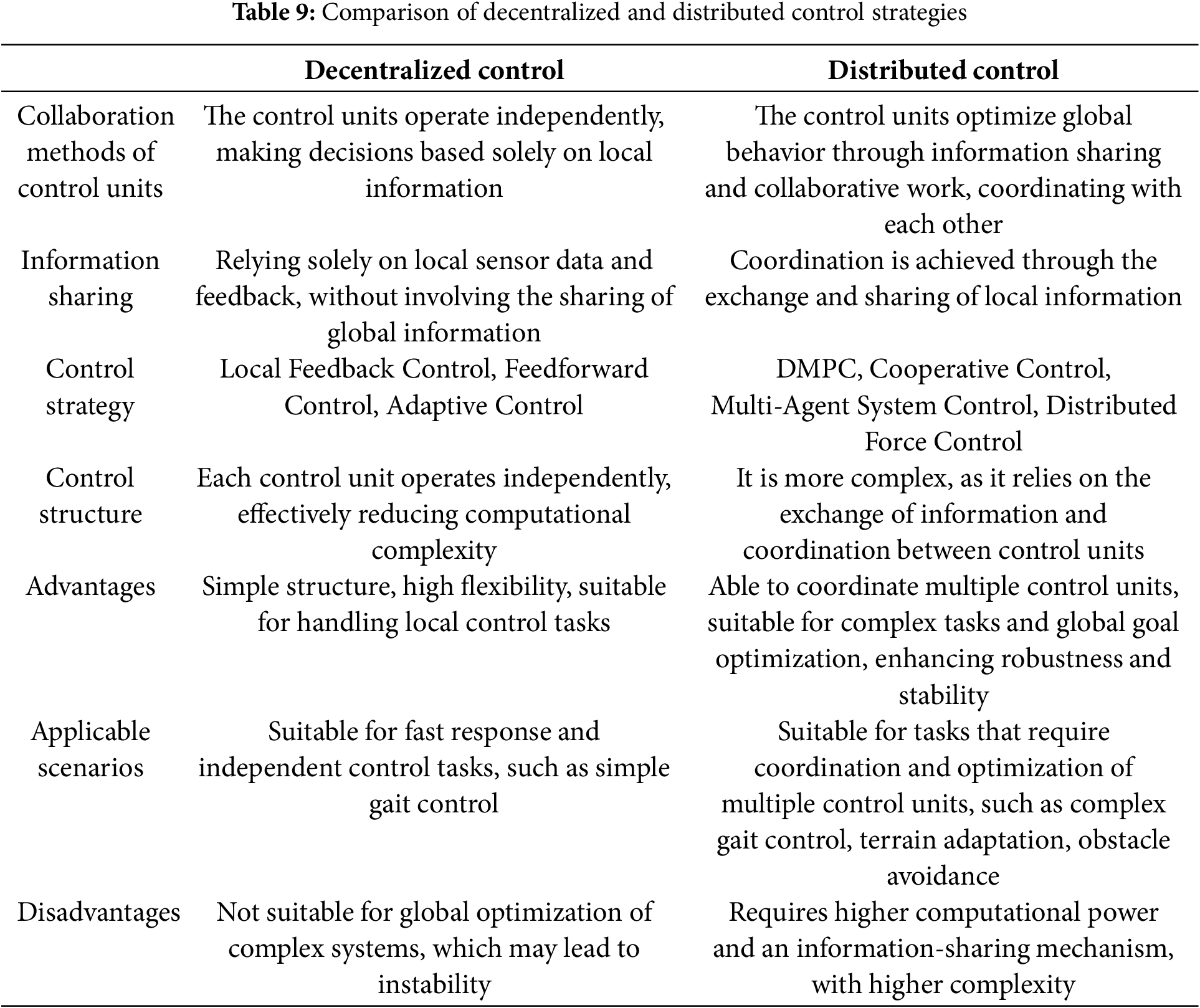
Decentralized control, where each leg is controlled independently, offers high flexibility and is well-suited for tasks requiring rapid response. However, it may perform poorly in global optimization and complex tasks. In contrast, distributed control leverages information exchange and cooperative control to efficiently coordinate multiple control units, making it ideal for complex motion control tasks, albeit at the cost of increased computational complexity. Both strategies have their respective application scenarios, and the choice of the most suitable control method depends on the complexity of the task and the performance requirements of the quadruped robot. Table 9 provides a summary of and comparison of these two control strategies.
3.4.1 Combination of ZMP and MPC
To enhance the dynamic performance, robustness, and multitasking capability of quadruped robots, researchers often optimize by combining multiple algorithms. In this optimization framework, MPC (Model Predictive Control) is used to calculate the optimal distribution of reaction forces over a longer time horizon based on a simplified dynamic model, while WBC (Whole-Body Control) utilizes the reaction force information generated by MPC to further compute joint torque, position, and velocity commands. This method has been successfully applied to the Mini-Cheetah quadruped robot, achieving excellent performance with a maximum running speed of 3.7 m/s after completing various gait tests. Through this fusion framework, not only is the dynamic model effectively simplified, but the computational complexity is significantly reduced. Experimental results demonstrate that the robot can smoothly transition between different gaits, fully proving the stability and effectiveness of this hybrid control strategy.
3.4.2 Integration of Reinforcement Learning with MPC
When performing highly dynamic tasks such as running and jumping, the application of methods like MPC (Model Predictive Control) is significantly constrained if the robot lacks high-precision environmental perception or accurate self-model support [133]. Additionally, end-to-end learning often exhibits low robustness when faced with drastic changes in tasks or environments and suffers from low sample efficiency. To address these challenges, researchers have proposed a method that combines MPC with learning-based techniques to better solve complex robotic motion tasks. Specifically, this method employs a simple linear function approximator to represent the control policy, and force distribution is computed via a Quadratic Programming (QP) process involving only 12 variables. Within this framework, MPC based on centroidal dynamics generates reference trajectory data, which is subsequently used to train the linear policy through imitation learning to minimize deviations from the reference trajectory. Thanks to this efficient computational approach, the controller has been successfully deployed on the Stoch3 robot, enabling it to stably execute highly dynamic tasks in both indoor and outdoor environments.
3.4.3 Integration of Reinforcement Learning with CPG
In addition to combining reinforcement learning (RL) with MPC to improve training efficiency and trajectory performance, researchers have also explored the integration of RL with Central Pattern Generator (CPG) models. Specifically, CPG models are used to represent open-loop motion strategies, while RL is employed to further optimize these strategies. Furthermore, in elastically actuated robots, another approach to achieving dynamic gaits involves using reflex-based controllers, whose parameters also require optimization.
This research framework applies not only to CPG controllers but also to reflex-based controllers. By leveraging learning-based methods to optimize the parameters of reflex controllers, automatic parameter adjustments can be achieved, thereby enhancing the system’s robustness and jumping performance.
To better understand the advantages and disadvantages of different integrated algorithms, Table 10 compares these algorithms. Fig. 22 illustrates the framework for gait planning and motion control structures in quadruped robots.
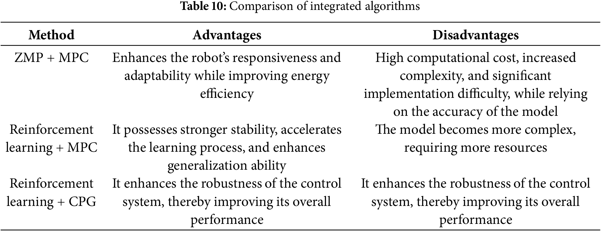
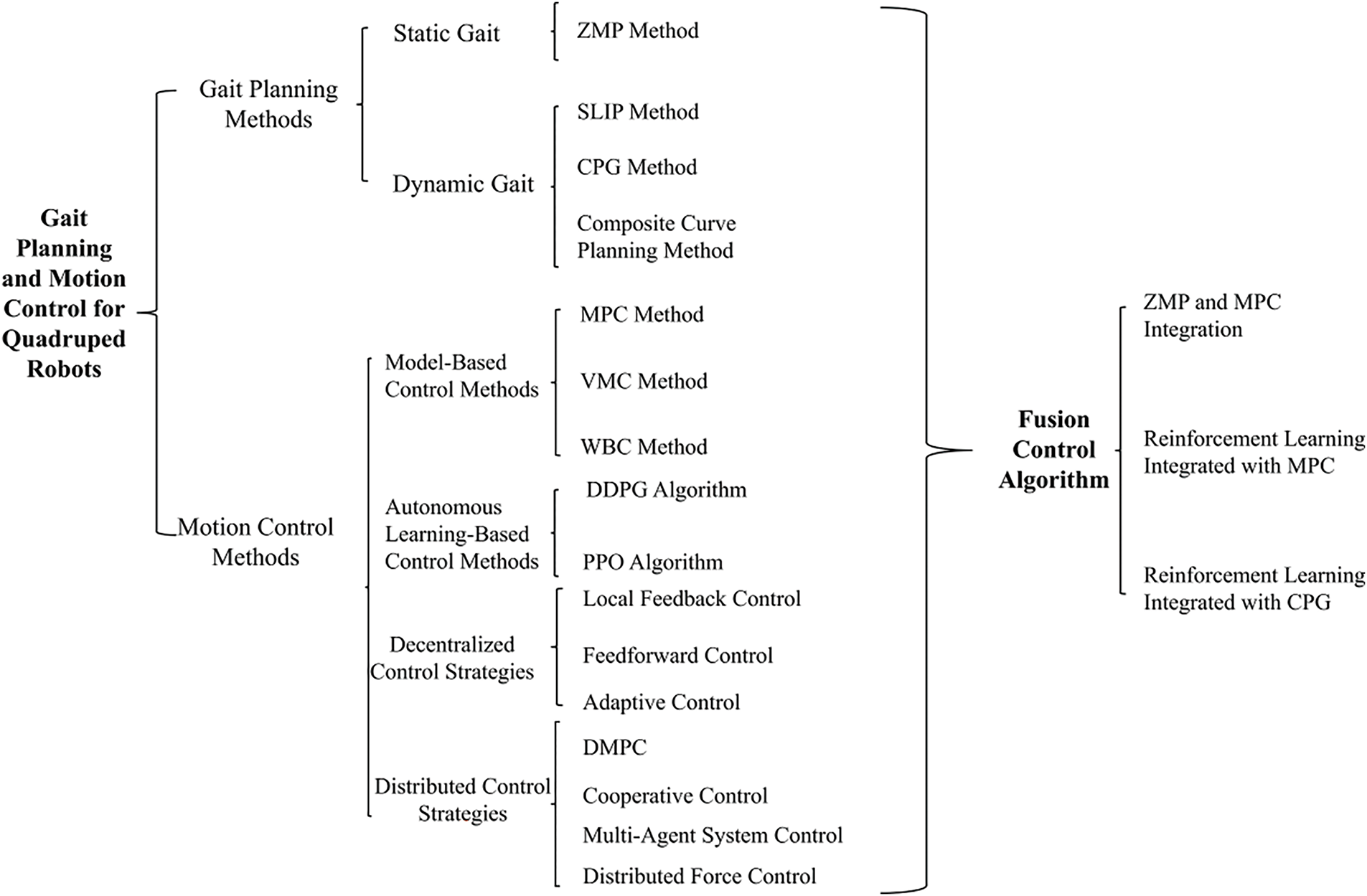
Figure 22: Structure block diagram of gait planning and motion control for quadruped robot
4 Challenges and Future Directions for Quadruped Robots
Quadruped robot technology is an interdisciplinary field that spans mechanical engineering, control engineering, computer engineering, and other areas [134]. The goal of quadruped robot research is to mimic, and even surpass, the movement capabilities and environmental adaptability of four-legged animals in nature [135]. According to existing literature, to bring robots closer to practical applications and fully exploit their flexible task capabilities, making their movements biomimetic to four-legged creatures, two major challenges remain [136]: First, quadruped robots are highly redundant systems with complex motion control; second, they must operate in dynamic and unpredictable environments.
Thus, achieving robust motion control for quadruped robots remains a significant challenge. Future research should focus on the following key aspects:
① High-strength mechanical design: During movement, the robot’s feet endure large impacts from the ground, which can be several times the robot’s static weight. New materials are not yet widely used in quadruped robots. Although active and passive compliance technologies can alleviate some of the shock, solid structural design remains crucial when robots need to carry weight [137]. Future quadruped robot research should focus on the application of high-strength lightweight materials and innovative mechanical structures to improve load bearing and shock-resistance performance.
② Multisensor data fusion: Integrating multiple sensors and effectively processing the data they provide is critical for enhancing a quadruped robot’s environmental awareness [138]. This involves solving issues such as sensor synchronization, calibration, and data fusion to ensure the robot can accurately perceive its surroundings.
③ Improving autonomy: The goal of quadruped robot development is to replace humans in performing tasks and to autonomously handle unexpected situations without human intervention [139]. Achieving higher levels of autonomy requires more than just basic motion planning; it necessitates in-depth research and optimization of control algorithms to ensure stronger autonomous decision-making and task execution capabilities.
④ More flexible movement modes: Quadruped animals in nature exhibit diverse and agile movement modes, including multiple gaits, jumping, and self-recovery after falls [140]. These capabilities enable them to adapt to various complex environments. An important future challenge is to enable quadruped robots to learn such flexible and agile movements and autonomously switch between different modes to adapt to real-world environments [141].
This paper systematically analyzes the main methods and key challenges in the field of gait trajectory planning and motion control for quadruped robots. As quadruped robots are increasingly applied in complex environments, gait planning and motion control have become critical technologies for enhancing their stability, flexibility, and adaptability. The paper first categorizes the gaits of quadruped robots, introducing the different characteristics of static and dynamic gaits. It then discusses the commonly used gait planning methods, as well as the unique advantages and applicable scenarios of each method. By analyzing these gait planning methods in-depth, this paper also proposes optimization objectives for quadruped robots in gait planning, including motion smoothness, maneuverability of the swing phase, and stability of foot contact. Particularly in complex dynamic environments, reasonable foot trajectory planning is crucial for improving the robot’s movement efficiency and reducing energy consumption. In terms of motion control, quadruped robots face numerous challenges, especially in ensuring stability and adaptability in complex terrains and uncertain environments. As research progresses, reinforcement learning-based control methods have gradually emerged, offering stronger autonomy and better environmental adaptability. However, to enable the widespread use of quadruped robots in practical tasks, many technical bottlenecks must still be overcome, including efficient control algorithms, multi-sensor data fusion, and decision-making capabilities, as well as stronger hardware designs.
Future research can focus on the following areas: further optimizing gait planning algorithms to improve their stability and efficiency in dynamic and complex environments; integrating artificial intelligence methods such as deep learning to enhance the robot’s autonomous perception and decision-making abilities; and, in hardware design, exploring lighter and more efficient driving systems to enhance the robot’s load-bearing capacity and motion performance. At the same time, interdisciplinary research, such as the combination of robotics and materials science, and control theory and artificial intelligence, will bring more technological breakthroughs to quadruped robots.
Research advancements in gait planning and motion control not only provide a solid technical foundation for the stability and flexibility of quadruped robots in complex environments but also address the enhancement of autonomy in dynamic tasks. With continuous innovations in algorithm optimization, artificial intelligence integration, and control methods, quadruped robots are poised to demonstrate greater environmental adaptability and task execution capabilities in increasingly diverse and challenging application scenarios.
Acknowledgement: The authors thank the Natural Science Basis Research Plan in Shaanxi Province of China and General Specialized Scientific Research Program of the Shaanxi Provincial Department of Education for supporting this study.
Funding Statement: This study is funded by the Natural Science Basis Research Plan in Shaanxi Province of China (Program No. 2023-JC-QN-0659) and General Specialized Scientific Research Program of the Shaanxi Provincial Department of Education (Program 23JK0349).
Author Contributions: The authors confirm contribution to the paper as follows: Draft manuscript preparation: Feihu Fan; Review the results and approve the final version of the manuscript: Sheng Dong; Creation of images and tables: Yinuo Chen; Collection of research concepts: Shangpeng Guo; Proofreading of article format: Jiayu Liu. All authors reviewed the results and approved the final version of the manuscript.
Availability of Data and Materials: All data generated or analyzed during this study are included in this published article.
Ethics Approval: Not applicable.
Conflicts of Interest: The authors declare no conflicts of interest to report regarding the present study.
Nomenclature
| ZMP | Zero Moment Point |
| CPG | Central Pattern Generator |
| SLIP | Spring Loaded Inverted Pendulum |
| COG | Center of Gravity |
| MPC | Model Predictive Control |
| VMC | Virtual Model Control |
| WBC | Whole-Body Control |
| QP | Quadratic Programming |
| NSP | Null Space Projection |
| HQP | Hierarchical Quadratic Programming |
| DRL | Deep Reinforcement Learning |
| DQN | Deep Q-Network |
| SAC | Soft-Actor-Critic |
| PG | Police Gradient |
| TD | Time Difference |
| DDPG | Deep Deterministic Policy Gradient |
| AC | Actor-Critic |
| PPO | Proximal Policy Optimization |
| TD3 | Twin Delayed Deep Deterministic Policy Gradient |
References
1. Tzafestas SG. Mobile robot control and navigation: a global overview. J Intell Robot Syst. 2018;91(1):35–58. doi:10.1007/s10846-018-0805-9. [Google Scholar] [CrossRef]
2. Ullah I, Adhikari D, Khan H, Anwar MS, Ahmad S, Bai X. Mobile robot localization: current challenges and future prospective. Comput Sci Rev. 2024;53(8):100651. doi:10.1016/j.cosrev.2024.100651. [Google Scholar] [CrossRef]
3. Chung W, Iagnemma K. Wheeled robots. Springer handbook of robotics. Berlin/Heidelberg, Germany: Springer; 2016. p. 575–94. doi:10.1007/978-3-540-30301-5_18. [Google Scholar] [CrossRef]
4. Zong C, Ji Z, Yu J, Yu H. An angle-changeable tracked robot with human-robot interaction in unstructured environments. Assem Autom. 2020;40(4):565–75. doi:10.1108/AA-11-2018-0231. [Google Scholar] [CrossRef]
5. Wang TM, Tao Y, Liu H. Current researches and future development trend of intelligent robot: a review. Int J Autom Comput. 2018;15(5):525–46. doi:10.1007/s11633-018-1115-1. [Google Scholar] [CrossRef]
6. Gupta S, Kumar A. A brief review of dynamics and control of underactuated biped robots. Adv Robot. 2017;31(12):607–23. doi:10.1080/01691864.2017.1308270. [Google Scholar] [CrossRef]
7. Coelho J, Ribeiro F, Dias B, Lopes G, Flores P. Trends in the control of hexapod robots: a survey. Robotics. 2021;10(3):100. doi:10.3390/robotics10030100. [Google Scholar] [CrossRef]
8. Fan Y, Pei Z, Wang C, Li M, Tang Z, Liu Q. A review of quadruped robots: structure, control, and autonomous motion. Adv Intell Syst. 2024;6(6):2300783. doi:10.1002/aisy.202300783. [Google Scholar] [CrossRef]
9. Ho T, Choi S, Lee S. Development of a biomimetic quadruped robot. J Bionic Eng. 2007;4(4):193–9. doi:10.1016/S1672-6529(07)60032-8. [Google Scholar] [CrossRef]
10. Yang K, Zhou L, Rong X, Li M, Tang Z, Liu Q. Onboard hydraulic system controller design for quadruped robot driven by gasoline engine. Mechatronics. 2018;52(4):36–48. doi:10.1016/j.mechatronics.2018.03.010. [Google Scholar] [CrossRef]
11. Xuefei L, Wenchang Z, Hang W, Chen W. Analysis and prospects of motion control algorithms for legged rescue robots. Chinese Med Equip J. 2022;43(1). doi:10.19745/j.1003-8868.2022020. [Google Scholar] [CrossRef]
12. McGhee RB. Some finite state aspects of legged locomotion. Math Biosci. 1968;2(1–2):67–84. doi:10.1016/0025-5564(68)90007-2. [Google Scholar] [CrossRef]
13. Frank AA. Automatic control systems for legged locomotion machines [dissertation]. Los Angeles, CA, USA: University of Southern California; 1968. [Google Scholar]
14. Mosher R. Test and evaluation of a versatile walking truck. In: Proceedings of Off-Road Mobility Research Symposium; 1968; Washington, DC, USA. p. 359–79. [Google Scholar]
15. Biswal P, Mohanty PK. Development of quadruped walking robots: a review. Ain Shams Eng J. 2021;12(2):2017–31. doi:10.1016/j.asej.2020.11.005. [Google Scholar] [CrossRef]
16. Li X, He J, Bian Z. Analysis and simulation of quadruped walking robot with hydraulic driving. In: Proceedings of the 5th International Conference on Mechanical, Automotive and Materials Engineering (CMAME); 2017; Piscataway, NJ, USA: IEEE. p. 154–57. [Google Scholar]
17. Raibert M, Blankespoor K, Nelson G, Playter R. Bigdog, the rough-terrain quadruped robot. IFAC. 2008;41(2):10822–5. doi:10.3182/20080706-5-KR-1001.01833. [Google Scholar] [CrossRef]
18. Gao FD. Complexity criteria for the preliminary design stage of walking robots. In: Proceedings of the International Design Engineering Technical Conferences and Computers and Information in Engineering Conference; 2017; New York, NY, USA: American Society of Mechanical Engineers. p. V05AT08A051. [Google Scholar]
19. Shkolnik A, Levashov M, Manchester IR, Tedrake R. Bounding on rough terrain with the LittleDog robot. Int J Robot. 2011;30(2):192–215. doi:10.1177/0278364910388315. [Google Scholar] [CrossRef]
20. Bouman A, Ginting MF, Alatur N, Palieri M, Fan DD, Touma T, et al. Autonomous spot: long-range autonomous exploration of extreme environments with legged locomotion. In: Proceedings of the 2020 IEEE/RSJ International Conference on Intelligent Robots and Systems (IROS); 2020; Piscataway, NJ, USA: IEEE. p. 2518–25. [Google Scholar]
21. Hutter M, Gehring C, Bloesch M, Hoepflinger MA, Remy CD, Siegwart R. StarlETH: a compliant quadrupedal robot for fast, efficient, and versatile locomotion. In: Adaptive mobile robotics. Singapore: World Scientific; 2012. p. 483–90. [Google Scholar]
22. Gehring C, Coros S, Hutter M, Bloesch M, Hoepflinger MA, Siegwart R. Control of dynamic gaits for a quadrupedal robot. In: Proceedings of the 2013 IEEE International Conference on Robotics and Automation; 2013; Piscataway, NJ, USA: IEEE. p. 3287–92. [Google Scholar]
23. Zhou C. Special issue “Legged Robots into the Real World”. Robotics. 2023;12(4):102. doi:10.3390/robotics12040102. [Google Scholar] [CrossRef]
24. Hussain K, Omar Z, Wang X, Adewale OO, Elnour M. Analysis and research of quadruped robot’s actuators: a review. Int J Mech Eng Robot Res. 2021;10(8):436–42. doi:10.18178/ijmerr.10.8.436-442. [Google Scholar] [CrossRef]
25. Kim D, Di Carlo J, Katz B, Bledt G, Kim S. Highly dynamic quadruped locomotion via whole-body impulse control and model predictive control. 2019. doi:10.48550/arXiv.1909.06586. [Google Scholar] [CrossRef]
26. Arena P, Pietro FD, Noce AL, Patanè L. Attitude control in the mini cheetah robot via MPC and reward-based feed-forward controller. IFAC-PapersOnLine. 2022;55(38):41–8. doi:10.1016/j.ifacol.2023.01.131. [Google Scholar] [CrossRef]
27. Katz B, Di Carlo J, Kim S. Mini cheetah: a platform for pushing the limits of dynamic quadruped control. In: Proceedings of the 2019 International Conference on Robotics and Automation (ICRA); 2019; Piscataway, NJ, USA: IEEE. p. 6295–301. [Google Scholar]
28. Bledt G, Powell MJ, Katz B, Di Carlo J, Wensing PM, Kim S. MIT cheetah 3: design and control of a robust, dynamic quadruped robot. In: Proceedings of the 2018 IEEE/RSJ International Conference on Intelligent Robots and Systems (IROS); 2018; Piscataway, NJ, USA: IEEE. p. 2245–52. [Google Scholar]
29. Di Carlo J. Software and control design for the MIT Cheetah quadruped robots [dissertation]. Cambridge, MA, USA: Massachusetts Institute of Technology; 2020. [Google Scholar]
30. Peng XB, Coumans E, Zhang T, Lee TW, Tan J, Levine S. Learning agile robotic locomotion skills by imitating animals. 2020. doi:10.48550/arXiv.2004.00784. [Google Scholar] [CrossRef]
31. Zhang G, Ma S, Shen Y, Li Y. A motion planning approach for nonprehensile manipulation and locomotion tasks of a legged robot. IEEE Trans Robot. 2020;36(3):855–74. doi:10.1109/TRO.2019.2961049. [Google Scholar] [CrossRef]
32. Wang P, Sun L. The stability analysis for quadruped bionic robot. In: Proceedings of the 2006 IEEE/RSJ International Conference on Intelligent Robots and Systems; 2006; Piscataway, NJ, USA: IEEE. p. 5238–42. [Google Scholar]
33. Romanov AM, Gyrichidi N, Romanov MP. Enabling navigation and mission-based control on a low-cost unitree Go1 air quadrupedal robot. 2023. doi:10.2139/ssrn.4584863. [Google Scholar] [CrossRef]
34. Askari M, Karakadioglu C, Ayhan F, Ayhan F, Ozcan O. MinIAQ-II: a miniature foldable quadruped with an improved leg mechanism. In: Proceedings of the 2017 IEEE International Conference on Robotics and Biomimetics (ROBIO); 2017; Piscataway, NJ, USA: IEEE. p. 19–25. [Google Scholar]
35. Yang C, Yuan K, Zhu Q, Yu W, Li Z. Multi-expert learning of adaptive legged locomotion. Sci Robot. 2020;5(49):eabb2174. doi:10.1126/scirobotics.abb2174. [Google Scholar] [CrossRef]
36. Xuan J, Luo H, Huang X, Sheng Y, Zhou H, Yu J. Motion performance analysis and application of quadruped robot for safety production supervision. In: Proceedings of the International Conference on Artificial Intelligence, Robotics, and Communication; 2023; Singapore: Springer Nature Singapore. p. 299–312. [Google Scholar]
37. Bellicoso CD, Bjelonic M, Wellhausen L, Holtmann K, Günther F, Tranzatto M, et al. Advances in real-world applications for legged robots. J Field Robot. 2018;35(8):1311–26. doi:10.1002/rob.21839. [Google Scholar] [CrossRef]
38. Hutter M, Gehring C, Lauber A, Gunther F, Bellicoso CD, Tsounis V, et al. Anymal-toward legged robots for harsh environments. Adv Robot. 2017;31(17):918–31. doi:10.1080/01691864.2017.1378591. [Google Scholar] [CrossRef]
39. Kolvenbach H, Wisth D, Buchanan R, Valsecchi G, Grandia R, Fallon M, et al. Towards autonomous inspection of concrete deterioration in sewers with legged robots. J Field Robot. 2020;37(8):1314–27. doi:10.1002/rob.21964. [Google Scholar] [CrossRef]
40. Kumar VR, Waldron KJ. A review of research on walking vehicles. Robot Rev 1. 1989;243–66. doi:10.1002/rob.10118. [Google Scholar] [CrossRef]
41. Li J, Wang J, Yang SX, Zhou K, Tang H. Gait planning and stability control of a quadruped robot. Comput Intell Neurosci. 2016;2016(1):9853070. doi:10.1155/2016/9853070. [Google Scholar] [CrossRef]
42. Zhang F, Teng S, Wang Y, Zhou K, Tang H. Design of bionic goat quadruped robot mechanism and walking gait planning. Int J Agric Biol Eng. 2020;13(5):32–9. doi:10.25165/j.ijabe.20201305.5769. [Google Scholar] [CrossRef]
43. Chen J, Xu K, Ding X. Adaptive gait planning for quadruped robot based on center of inertia over rough terrain. Biomimetic Intell Robot. 2022;2(1):100031. doi:10.1016/j.birob.2021.100031. [Google Scholar] [CrossRef]
44. Li Z, Song Y, Zhang X, Peng X, Xu N. Modeling of walking-gait parameters and walking strategy for quadruped robots. Appl Sci. 2023;13(12):6876. doi:10.3390/app13126876. [Google Scholar] [CrossRef]
45. Chen JP, San HJ, Wu X, Peng X, Xu N. Structural design and gait research of a new bionic quadruped robot. Proc Inst Mech Eng Part B: J Eng Manuf. 2022;236(14):1912–22. doi:10.1177/0954405421995663. [Google Scholar] [CrossRef]
46. Divandari M, Ghabi D, Kalteh AA. Stability prediction of quadruped robot movement using classification methods and principal component analysis. Adv Electr Electron Eng. 2023;21(4):295–304. doi:10.15598/aeee.v21i4.5215. [Google Scholar] [CrossRef]
47. Joseph T, Shaikh A, Sarode M, Rao YS. Quadruped robots: gait analysis and control. In: Proceedings of the 2020 IEEE 17th India Council International Conference (INDICON); 2020; Piscataway, NJ, USA: IEEE. p. 1–6. [Google Scholar]
48. Jia Y, Luo X, Han B, Liang G, Zhao J, Zhao Y. Stability criterion for dynamic gaits of quadruped robot. Appl Sci. 2018;8(12):2381. doi:10.3390/app8122381. [Google Scholar] [CrossRef]
49. Hao Q, Wang Z, Wang J, Chen G. Stability-guaranteed and high terrain adaptability static gait for quadruped robots. Sensors. 2020;20(17):4911. doi:10.3390/s20174911. [Google Scholar] [CrossRef]
50. Bi J, Chen T, Rong X, Chen G. Efficient dynamic locomotion of quadruped robot via adaptive diagonal gait. J Bionic Eng. 2024;21(1):126–36. doi:10.1007/s42235-023-00432-z. [Google Scholar] [CrossRef]
51. Vincelette A. The characteristics, distribution, function, and origin of alternative lateral horse gaits. Animals. 2023;13(16):2557. doi:10.3390/ani13162557. [Google Scholar] [CrossRef]
52. Fukui T, Fujisawa H, Otaka K, Fukuoka Y. Autonomous gait transition and galloping over unperceived obstacles of a quadruped robot with CPG modulated by vestibular feedback. Robot Auton Syst. 2019;111:1–19. doi:10.1016/j.robot.2018.10.002. [Google Scholar] [CrossRef]
53. Hao X, Wei L, Qiao Y, Fukuoka Y. Bounding gait control of a parallel quadruped robot. Ind Robot: Int J Robot Res Appl. 2023;50(6):888–99. doi:10.1108/IR-12-2022-0321. [Google Scholar] [CrossRef]
54. Zeng X, Zhang S, Zhang H, Li X, Zhou H, Fu Y. Leg trajectory planning for quadruped robots with high-speed trot gait. Appl Sci. 2019;9(7):1508. doi:10.3390/app9071508. [Google Scholar] [CrossRef]
55. Vukobratović M, Borovac B. Zero-moment point—thirty five years of its life. Int J HR. 2004;1(1):157–73. doi:10.1142/S0219843604000083. [Google Scholar] [CrossRef]
56. Kimura H, Fukuoka Y, Hada Y, Takase K. Three-dimensional adaptive dynamic walking of a quadruped—rolling motion feedback to CPGs controlling pitching motion. In: Proceedings of the 2002 IEEE International Conference on Robotics and Automation (Cat. No. 02CH37292); 2002; Piscataway, NJ, USA: IEEE. p. 2228–33. [Google Scholar]
57. Raibert MH. Hopping in legged systems—modeling and simulation for the two-dimensional one-legged case. IEEE Trans Syst, Man, Cybern. 1984;3:451–63. doi:10.1109/TSMC.1984.6313238. [Google Scholar] [CrossRef]
58. Dinçer Ü, Çevik M. Improved trajectory planning of an industrial parallel mechanism by a composite polynomial consisting of Bézier curves and cubic polynomials. Mech Mach Theory. 2019;132(5):248–63. doi:10.1016/j.mechmachtheory.2018.11.009. [Google Scholar] [CrossRef]
59. Wigler AW, Farshidian F, Neunert M, Pardo D, Buchli J. Online walking motion and foothold optimization for quadruped locomotion. In: Proceedings of the 2017 IEEE International Conference on Robotics and Automation (ICRA); 2017; Piscataway, NJ, USA: IEEE. p. 5308–13. [Google Scholar]
60. Globisz A, Krawczyk D. Determination of center of gravity location and ground reaction forces for 4-legged walking robot. In: Proceedings of the 2016 11th France-Japan & 9th Europe-Asia Congress on Mechatronics (MECATRONICS)/17th International Conference on Research and Education in Mechatronics (REM); 2016; Piscataway, NJ, USA: IEEE. p. 158–63. [Google Scholar]
61. Nakamura Y, Ghodoussi M. A computational scheme of closed link robot dynamics derived by D’Alembert principle. In: Proceedings of the 1988 IEEE International Conference on Robotics and Automation; 1988; Piscataway NJ, USA: IEEE. p. 1354–60. [Google Scholar]
62. Kim JH. Multi-axis force-torque sensors for measuring zero-moment point in humanoid robots: a review. IEEE Sens J. 2019;20(3):1126–41. doi:10.1109/JSEN.2019.2947719. [Google Scholar] [CrossRef]
63. Meng X, Liu W, Tang L, Lu Z, Lin H, Fang J. Trot gait stability control of small quadruped robot based on MPC and ZMP methods. Processes. 2023;11(1):252. doi:10.3390/pr11010252. [Google Scholar] [CrossRef]
64. Hooper SL. Central pattern generators. Curr Biol. 2000;10(5):R176–9. doi:10.1016/S0960-9822(00)00367-5. [Google Scholar] [CrossRef]
65. Bellegarda G, Ijspeert A. CPG-RL: learning central pattern generators for quadruped locomotion. IEEE Robot Automation Lett. 2022;7(4):12547–54. doi:10.1109/LRA.2022.3218167. [Google Scholar] [CrossRef]
66. Ma Z, Liang Y, Tian H. Research on gait planning algorithm of quadruped robot based on central pattern generator. In: Proceedings of the 2020 39th Chinese Control Conference (CCC); 2020; Piscataway, NJ, USA: IEEE. p. 3948–53. [Google Scholar]
67. Liu J, Pu J, Gu J. Central pattern generator based crawl gait control for quadruped robot. In: Proceedings of the 2016 IEEE International Conference on Information and Automation (ICIA); 2016; Piscataway, NJ, USA: IEEE. p. 956–62. [Google Scholar]
68. Lodi M, Shilnikov A, Storace M. Design of synthetic central pattern generators producing desired quadruped gaits. IEEE Trans Circuits Syst I: Regul Papers. 2017;65(3):1028–39. doi:10.1109/TCSI.2017.2759320. [Google Scholar] [CrossRef]
69. Wei S, Wu H, Liu L, Zhang Y, Chen J, Li Q. A CPG-based gait planning and motion performance analysis for quadruped robot. Ind Robot. 2022;49(4):779–97. doi:10.1108/IR-08-2021-0181. [Google Scholar] [CrossRef]
70. Liu C, Xia L, Zhang C, Chen Q. Multi-layered CPG for adaptive walking of quadruped robots. J Bionic Eng. 2018;15(2):341–55. doi:10.1007/s42235-018-0026-8. [Google Scholar] [CrossRef]
71. Soyguder S, Alli H. Computer simulation and dynamic modeling of a quadrupedal pronking gait robot with SLIP model. Comput Electr Eng. 2012;38(1):161–74. doi:10.1016/j.compeleceng.2011.11.007. [Google Scholar] [CrossRef]
72. Yılmaz MK. Control of quadruped walking behavior through an embedding of spring loaded inverted pendulum template [dissertation]. Ankara, Turkey: Middle East Technical University; 2022. [Google Scholar]
73. Chen J, San H. Structure design and gait transition stability of quadruped robot. In: 13th International Conference on Quality, Reliability, Risk, Maintenance, and Safety Engineering (QR2MSE 2023); 2023; Kunming, China. p. 328–36. doi:10.1049/icp.2023.1661. [Google Scholar] [CrossRef]
74. Gu J, Li L, Zhou S, Zhang W. Research on foot trajectory planning of quadruped robot: based on high degree polynomial curve. In: Proceedings of the 2022 4th International Conference on Robotics, Intelligent Control and Artificial Intelligence; 2022; New York, NY, USA: Association for Computing Machinery. p. 87–94. [Google Scholar]
75. Pedro GDG, Bermudez G, Medeiros VS, Cruz Neto HJ, Barros LGD, Pessin G, et al. Quadruped robot control: an approach using body planar motion control, legs impedance control and Bézier curves. Sensors. 2024;24(12):3825. doi:10.3390/s24123825. [Google Scholar] [CrossRef]
76. Abdulwahab AH, Mazlan AZA, Hawary AF, Hadi NH. Quadruped robots mechanism, structural design, energy, gait, stability, and actuators: a review study. Int J Mech Eng Robot Res. 2023;12(6):385–95. doi:10.18178/ijmerr.12.6.385-395. [Google Scholar] [CrossRef]
77. Li M, Liu Z, Wang M, Pang G, Zhang H. Design of a parallel quadruped robot based on a novel intelligent control system. Appl Sci. 2022;12(9):4358. doi:10.3390/app12094358. [Google Scholar] [CrossRef]
78. Wang J, Chatzinikolaidis I, Mastalli C, Wolfslag W, Xin G, Tonneau S, et al. Automatic gait pattern selection for legged robots. In: Proceedings of the 2020 IEEE/RSJ International Conference on Intelligent Robots and Systems (IROS); 2020; Piscataway, NJ, USA: IEEE. p. 3990–7. [Google Scholar]
79. Chai H, Li Y, Song R, Wolfslag W, Xin G, Tonneau S, et al. A survey of the development of quadruped robots: joint configuration, dynamic locomotion control method and mobile manipulation approach. Biomim Intell Robot. 2022;2(1):100029. doi:10.1016/j.birob.2021.100029. [Google Scholar] [CrossRef]
80. Taheri H, Mozayani N. A study on quadruped mobile robots. Mech Mach Theory. 2023;190:105448. doi:10.1016/j.mechmachtheory.2023.105448. [Google Scholar] [CrossRef]
81. Chi W, Jiang X, Zheng Y. A linearization of centroidal dynamics for the model-predictive control of quadruped robots. In: Proceedings of the 2022 International Conference on Robotics and Automation (ICRA); 2022; Piscataway, NJ, USA: IEEE. p. 4656–63. [Google Scholar]
82. Chen G, Guo S, Hou B, Wang J. Virtual model control for quadruped robots. IEEE Access. 2020;8:140736–51. doi:10.1109/ACCESS.2020.3013434. [Google Scholar] [CrossRef]
83. Fahmi S, Mastalli C, Focchi M, Wang J. Passive whole-body control for quadruped robots: experimental validation over challenging terrain. IEEE Robot Autom Lett. 2019;4(3):2553–60. doi:10.1109/LRA.2019.2908502. [Google Scholar] [CrossRef]
84. Di Carlo J, Wensing PM, Katz B, Bledt G, Kim S. Dynamic locomotion in the MIT Cheetah 3 through convex model-predictive control. In: Proceedings of the 2018 IEEE/RSJ International Conference on Intelligent Robots and Systems (IROS); 2018; Piscataway, NJ, USA: IEEE. p. 1–9. [Google Scholar]
85. Grandia R, Farshidian F, Dosovitskiy A, Bledt G, Kim S. Frequency-aware model predictive control. IEEE Robot Autom Lett. 2019;4(2):1517–24. doi:10.1109/LRA.2019.2895882. [Google Scholar] [CrossRef]
86. Xin G, Mistry M. Optimization-based dynamic motion planning and control for quadruped robots. Nonlinear Dyn. 2024;112(9):7043–56. doi:10.1007/s11071-024-09445-7. [Google Scholar] [CrossRef]
87. Kim DH, Park JH. Reduced model predictive control toward highly dynamic quadruped locomotion. IEEE Access. 2024;12:20003–18. doi:10.1109/ACCESS.2024.3360479. [Google Scholar] [CrossRef]
88. Zhang Z, Chang X, Ma H, An H, Lang L. Model predictive control of quadruped robot based on reinforcement learning. Appl Sci. 2022;13(1):154. doi:10.3390/app13010154. [Google Scholar] [CrossRef]
89. Pratt J, Chew C-M, Torres A, Dilworth P, Pratt G. Virtual model control: an intuitive approach for bipedal locomotion. Int J Robot Res. 2001;20(2):129–43. doi:10.1177/02783640122067309. [Google Scholar] [CrossRef]
90. Pratt J, Dilworth P, Pratt G. Virtual model control of a bipedal walking robot. In: Proceedings of the 1997 IEEE International Conference on Robotics and Automation; 1997; Piscataway, NJ, USA: IEEE. p. 193–8. [Google Scholar]
91. Hua Z, Rong X, Li Y, Chai H, Zhang S. Active compliance control on the hydraulic quadruped robot with passive compliant servo actuator. IEEE Access. 2019;7:163449–60. doi:10.1109/ACCESS.2019.2951830. [Google Scholar] [CrossRef]
92. Xie H, Ahmadi M, Shang J, Luo Z. An intuitive approach for quadruped robot trotting based on virtual model control. Proc Inst Mech Eng, Part I: J Syst Control Eng. 2015;229(4):342–55. doi:10.1177/0959651814562620. [Google Scholar] [CrossRef]
93. Chen G, Hou B, Guo S, Wang J. Dynamic balance and trajectory tracking control of quadruped robots based on virtual model control. In: Proceedings of the 2020 39th Chinese Control Conference (CCC); 2020; Piscataway, NJ, USA: IEEE. p. 3771–6. [Google Scholar]
94. Khatib O. A unified approach for motion and force control of robot manipulators: the operational space formulation. IEEE J Robot Autom. 1987;3(1):43–53. doi:10.1109/JRA.1987.1087068. [Google Scholar] [CrossRef]
95. Khatib O, Sentis L, Park J, Warren J. Whole-body dynamic behavior and control of human-like robots. Int J HR. 2004;1(1):29–43. doi:10.1142/S0219843604000058. [Google Scholar] [CrossRef]
96. Liu M, Xu F, Jia K, Yang Q, Tang C. A stable walking strategy of quadruped robot based on foot trajectory planning. In: Proceedings of the 2016 3rd International Conference on Information Science and Control Engineering (ICISCE); 2016; Piscataway NJ, USA: IEEE. p. 799–803. [Google Scholar]
97. Sombolestan M, Nguyen Q. Hierarchical adaptive loco-manipulation control for quadruped robots. In: Proceedings of the 2023 IEEE International Conference on Robotics and Automation (ICRA); 2023; Piscataway, NJ, USA: IEEE. p. 12156–62. [Google Scholar]
98. Dietrich A, Ott C, Albu-Schäffer A. An overview of null space projections for redundant, torque-controlled robots. Int J Robot Res. 2015;34(11):1385–400. doi:10.1177/0278364914566516. [Google Scholar] [CrossRef]
99. Tian D, Gao J, Shi X, Lu Y, Liu C. Vertical jumping for legged robot based on quadratic programming. Sensors. 2021;21(11):3679. doi:10.3390/s21113679. [Google Scholar] [CrossRef]
100. Gehring C, Bellicoso CD, Fankhauser P, Fankhauser P, Coros S, Hutter M. Quadrupedal locomotion using trajectory optimization and hierarchical whole body control. In: Proceedings of the 2017 IEEE International Conference on Robotics and Automation (ICRA); 2017; Piscataway, NJ, USA: IEEE. p. 4788–94. [Google Scholar]
101. Rudin N, Hoeller D, Reist P, Hutter M. Learning to walk in minutes using massively parallel deep reinforcement learning. In: Proceedings of the Conference on Robot Learning; 2022; Auckland, New Zealand. Palo Alto, CA, USA: PMLR. p. 91–100. [Google Scholar]
102. Bellegarda G, Nguyen C, Nguyen Q. Robust quadruped jumping via deep reinforcement learning. Robot Auton Syst. 2024;182:104799. doi:10.48550/arXiv.2011.07089. [Google Scholar] [CrossRef]
103. Ernst D, Louette A. Introduction to reinforcement learning. 2024. doi:10.48550/arXiv.2408.07712. [Google Scholar] [CrossRef]
104. Li Y. Deep reinforcement learning: an overview. 2017. doi:10.48550/arXiv.1701.07274. [Google Scholar] [CrossRef]
105. Mousavi SS, Schukat M, Howley E. Deep reinforcement learning: an overview. In: Proceedings of the SAI Intelligent Systems Conference (IntelliSys); 2018; London, UK. Berlin, Germany: Springer International Publishing. p. 426–40. [Google Scholar]
106. François-Lavet V, Henderson P, Islam R, Bellemare MG, Pineau J. An introduction to deep reinforcement learning. Found Trends® Mach Learn. 2018;11(3–4):219–354. doi:10.1561/2200000071. [Google Scholar] [CrossRef]
107. Wang X, Wang S, Liang X, Zhao D, Huang J, Xu X, et al. Deep reinforcement learning: a survey. IEEE Trans Neural Netw Learn Syst. 2022;35(4):5064–78. doi:10.1109/TNLS.2022.3207346. [Google Scholar] [CrossRef]
108. Wang X, Gu Y, Cheng Y, Liu A, Chen CP. Approximate policy-based accelerated deep reinforcement learning. IEEE Trans Neural Netw Learn Syst. 2019;31(6):1820–30. doi:10.1109/TNLS.2019.2927227. [Google Scholar] [CrossRef]
109. Zhong C, Lu Z, Gursoy MC, Velipasalar S. A deep actor-critic reinforcement learning framework for dynamic multichannel access. IEEE Trans Cogn Commun Netw. 2019;5(4):1125–39. doi:10.1109/TCCN.2019.2952909. [Google Scholar] [CrossRef]
110. Li SE. Deep reinforcement learning. In: Reinforcement learning for sequential decision and optimal control. Singapore: Springer Nature Singapore; 2023. p. 365–402. [Google Scholar]
111. Tsounis V, Alge M, Lee J, Farshidian F, Hutter M. Deepgait: planning and control of quadrupedal gaits using deep reinforcement learning. IEEE Robot Autom Lett. 2020;5(2):3699–706. doi:10.1109/LRA.2020.2979660. [Google Scholar] [CrossRef]
112. Lee J, Hwangbo J, Hutter M. Robust recovery controller for a quadrupedal robot using deep reinforcement learning. 2019. doi:10.13140/RG.2.2.11697.39523. [Google Scholar] [CrossRef]
113. Apostolidis E, Adamantidou E, Metsai AI, Mezaris V, Patras I. AC-SUM-GAN: connecting actor-critic and generative adversarial networks for unsupervised video summarization. IEEE Trans Circuits Syst Video Technol. 2021;31(8):3278–92. doi:10.1109/TCSVT.2020.3037883. [Google Scholar] [CrossRef]
114. Neri F, Liu X, Yue P, Yue P, Zhang G. Deep deterministic policy gradient with constraints for gait optimisation of biped robots. Integr Comput Aided Eng. 2024;31(2):139–56. doi:10.3233/ICA-230724. [Google Scholar] [CrossRef]
115. Li Y, Chen Z, Wu C, Mao H, Sun P. A hierarchical framework for quadruped robots gait planning based on DDPG. Biomimetics. 2023;8(5):382. doi:10.3390/biomimetics8050382. [Google Scholar] [CrossRef]
116. Li C, Zhu X, Ruan X, Liu X, Zhang S. Gait learning reproduction for quadruped robots based on experience evolution proximal policy optimization. J Shanghai Jiaotong Univ (Sci). 2023;6(5):61. doi:10.1007/s12204-023-2666-z. [Google Scholar] [CrossRef]
117. Zhang L, Shen L, Yang L, Chen S, Yuan B, Wang X, et al. Penalized proximal policy optimization for safe reinforcement learning. 2022. doi:10.48550/arXiv.2205.11814. [Google Scholar] [CrossRef]
118. Zashchitin R, Dobriborsci D. A study on the energy efficiency of various gaits for quadruped robots: generation and evaluation. In: Proceedings of the 20th International Conference on Informatics in Control, Automation and Robotics (ICINCO 2023); 2023; Singapore: Springer Nature Singapore. p. 311–9. [Google Scholar]
119. Zhang Y, Zeng J, Sun H, Sun H, Hashimoto K. Dual-layer reinforcement learning for quadruped robot locomotion and speed control in complex environments. Appl Sci. 2024;14(19):8697. doi:10.3390/app14198697. [Google Scholar] [CrossRef]
120. Amaike H, Fukuhara A, Kano T, Ishiguro A. Decentralized control mechanism for limb steering in quadruped robot walking. Adv Robot. 2024;38(16):1124–40. doi:10.1080/01691864.2024.2376030. [Google Scholar] [CrossRef]
121. Sartoretti G, Paivine W, Shi Y, Wu Y, Choset H. Distributed learning of decentralized control policies for articulated mobile robots. IEEE Trans Robot. 2019;35(5):1109–22. doi:10.1109/TRO.2019.2922493. [Google Scholar] [CrossRef]
122. Kamidi VR, Kim J, Fawcett RT, Ames AD, Hamed KA. Distributed quadratic programming-based nonlinear controllers for periodic gaits on legged robots. IEEE Control Syst Lett. 2022;6:2509–14. doi:10.1109/LCSYS.2022.3167795. [Google Scholar] [CrossRef]
123. Imran BM, Fawcett RT, Kim J, Leonessa A, Akbari Hamed K. A distributed layered planning and control algorithm for teams of quadrupedal robots: an obstacle-aware nonlinear MPC approach. J Dyn Syst Meas Control. 2025;147(3):031006. doi:10.1115/1.4066632. [Google Scholar] [CrossRef]
124. Fukuhara A, Koizumi Y, Suzuki S, Kano T, Ishiguro A. Decentralized control mechanism for body-limb coordination in quadruped running. Adapt Behav. 2020;28(3):151–64. doi:10.1177/1059712319865180. [Google Scholar] [CrossRef]
125. Vasconcelos R, Hauser S, Dzeladini F, Mutlu M, Horvat T, Melo K, et al. Active stabilization of a stiff quadruped robot using local feedback. In: Proceedings of the 2017 IEEE/RSJ International Conference on Intelligent Robots and Systems (IROS); 2017; Piscataway, NJ, USA: IEEE. p. 4903–10. [Google Scholar]
126. Kurazume R, Yoneda K, Hirose S. Feedforward and feedback dynamic trot gait control for quadruped walking vehicle. In: Proceedings 2001 ICRA. IEEE International Conference on Robotics and Automation; 2001; Seoul, Republic of Korea. p. 3172–80. doi:10.1109/ROBOT.2001.933105. [Google Scholar] [CrossRef]
127. Massi E, Vannucci L, Albanese U, Capolei MC, Vandesompele A, Urbain G, et al. Combining evolutionary and adaptive control strategies for quadruped robotic locomotion. Front Neurorobot. 2019;13:71. doi:10.3389/fnbot.2019.00071. [Google Scholar] [CrossRef]
128. Amatucci L, Turrisi G, Bratta A, Barasuol V, Semini C. Accelerating model predictive control for legged robots through distributed optimization. 2024. doi:10.48550/arXiv.2403.11742. [Google Scholar] [CrossRef]
129. Liu K, Dong L, Tan X, Zhang W, Zhu L. Optimization-based flocking control and MPC-based gait synchronization control for multiple quadruped robots. IEEE Robot Autom Lett. 2024;9(2):1929–36. doi:10.1109/LRA.2024.3350372. [Google Scholar] [CrossRef]
130. Kim J, Fawcett RT, Kamidi VR, Ames AD, Hamed KA. Layered control for cooperative locomotion of two quadrupedal robots: centralized and distributed approaches. IEEE Trans Robot. 2023;39(6):4728–48. doi:10.1109/TRO.2023.3319896. [Google Scholar] [CrossRef]
131. Liu Q, Guo J, Lin S, Ma S, Zhu J, Li Y. MASQ: multi-agent reinforcement learning for single quadruped robot locomotion. 2024. doi:10.48550/arXiv.2408.13759. [Google Scholar] [CrossRef]
132. Biswal P, Mohanty PK. Modeling and effective foot force distribution for the legs of a quadruped robot. Robotica. 2021;39(8):1504–17. doi:10.1017/S0263574720001307. [Google Scholar] [CrossRef]
133. Shi Y, Wang P, Li M, Wang X, Jiang Z, Li Z. Model predictive control for motion planning of quadrupedal locomotion. In: Proceedings of the 2019 IEEE 4th International Conference on Advanced Robotics and Mechatronics (ICARM); 2019; Piscataway, NJ, USA: IEEE. p. 87–92. [Google Scholar]
134. Meng X, Wang S, Cao Z, Zhang L. A review of quadruped robots and environment perception. In: Proceedings of the 2016 35th Chinese Control Conference (CCC); 2016; New York, NY, USA: IEEE. p. 6350–6. [Google Scholar]
135. Hamrani A, Rayhan MM, Mackenson T, McDaniel D, Lagos L. Smart quadruped robotics: a systematic review of design, control, sensing and perception. Adv Robot. 2025;39(1):3–29. doi:10.1080/01691864.2024.2411684. [Google Scholar] [CrossRef]
136. Gong D, Wang P, Zhao S, Du L, Duan Y. Bionic quadruped robot dynamic gait control strategy based on twenty degrees of freedom. IEEE/CAA J Automatica Sin. 2017;5(1):382–8. doi:10.1109/JAS.2017.7510790. [Google Scholar] [CrossRef]
137. Shi Y, Li S, Guo M, Yang Y, Xia D, Luo X. Structural design, simulation and experiment of quadruped robot. Appl Sci. 2021;11(22):10705. doi:10.3390/app112210705. [Google Scholar] [CrossRef]
138. Chen G, Hong L. Research on environment perception system of quadruped robots based on LiDAR and vision. Drones. 2023;7(5):329. doi:10.3390/drones7050329. [Google Scholar] [CrossRef]
139. Gilroy S, Lau D, Yang L, Izaguirre E, Biermayer K, Xiao A, et al. Autonomous navigation for quadrupedal robots with optimized jumping through constrained obstacles. In: Proceedings of the 2021 IEEE 17th International Conference on Automation Science and Engineering (CASE); 2021; Piscataway, NJ, USA: IEEE. p. 2132–9. [Google Scholar]
140. Shafiee M, Bellegarda G, Ijspeert A. Manyquadrupeds: learning a single locomotion policy for diverse quadruped robots. In: Proceedings of the 2024 IEEE International Conference on Robotics and Automation (ICRA); 2024; Piscataway, NJ, USA: IEEE. p. 3471–7. [Google Scholar]
141. He JY, Shao JP, Sun GT, Shao X. Survey of quadruped robots coping strategies in complex situations. Electronics. 2019;8(12):1414. doi:10.3390/electronics8121414. [Google Scholar] [CrossRef]
Cite This Article
 Copyright © 2025 The Author(s). Published by Tech Science Press.
This work is licensed under a Creative Commons Attribution 4.0 International License , which permits unrestricted use, distribution, and reproduction in any medium, provided the original work is properly cited.
 Downloads
 Citation Tools